
Applications of Linear Functions
Rates of Change
Linear functions apply to real world problems that involve a constant rate.Learning Objectives
Apply linear equations to solve problems about rates of changeKey Takeaways
Key Points
- If you know a real-world problem is linear, such as the distance you travel when you go for a jog, you can graph the function and make some assumptions with only two points.
- The slope of a function is the same as the rate of change for the dependent variable [latex](y)[/latex]. For instance, if you're graphing distance vs. time, then the slope is how fast your distance is changing with time, or in other words, your velocity.
Key Terms
- rate of change: Ratio between two related quantities that are changing.
- linear equation: A polynomial equation of the first degree (such as [latex]x=2y-7[/latex]).
- slope: The ratio of the vertical and horizontal distances between two points on a line; zero if the line is horizontal, undefined if it is vertical.
Rate of Change
Linear equations often include a rate of change. For example, the rate at which distance changes over time is called velocity. If two points in time and the total distance traveled is known the rate of change, also known as slope, can be determined. From this information, a linear equation can be written and then predictions can be made from the equation of the line. If the unit or quantity in respect to which something is changing is not specified, usually the rate is per unit of time. The most common type of rate is "per unit of time", such as speed, heart rate and flux. Ratios that have a non-time denominator include exchange rates, literacy rates, and electric field (in volts/meter). In describing the units of a rate, the word "per" is used to separate the units of the two measurements used to calculate the rate (for example a heart rate is expressed "beats per minute").Rate of Change: Real World Application
Example
An athlete begins he normal practice for the next marathon during the evening. At 6:00 pm he starts to run and leaves his home. At 7:30 pm, the athlete finishes the run at home and has run a total of 7.5 miles. How fast was his average speed over the course of the run? The rate of change is the speed of his run; distance over time. Therefore, the two variables are time [latex](x)[/latex] and distance [latex](y)[/latex]. The first point is at his house, where his watch read 6:00 pm. This is the beginning time so let's set it to [latex]0[/latex]. So our first point is [latex](0,0)[/latex] because he did not run anywhere yet. Let's think about our time in hours. Our second point is [latex]1.5[/latex] hours later, and we ran [latex]7.5[/latex] miles. The second point is [latex](1.5,7.5)[/latex]. Our speed (rate of change) is simply the slope of the line connecting the two points. The slope, given by: [latex]m = \frac{y_{2}-y_{1}}{x_{2}-x_{1}}[/latex] becomes [latex]m = \frac{7.5}{1.5}=5 [/latex] miles per hour.Example: Graph the line illustrating speed
To graph this line, we need the [latex]y[/latex]-intercept and the slope to write the equation. The slope was [latex]5[/latex] miles per hour and since the starting point was at [latex](0,0)[/latex], the [latex]y[/latex]-intercept is [latex]0[/latex]. So our final function is [latex]y=5x[/latex].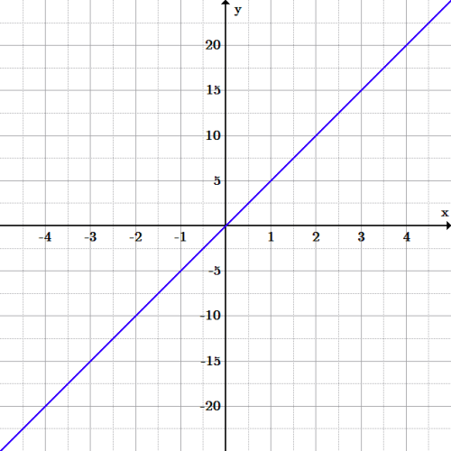 Distance and time graph: The graph of [latex]y=5x[/latex]. The two variables are time [latex](x)[/latex] and distance [latex](y)[/latex]. The rate the runner runs is [latex]5[/latex] miles per hour. Using the graph, predictions can be made assuming that his average speed remains the same.
With this new function, we can now answer some more questions.
- How many miles did he run after the first half hour? Using the equation, if [latex]x=\frac{1}{2}[/latex], solve for [latex]y[/latex]. If [latex]y=5x[/latex], then [latex]y=5(0.5)=2.5[/latex] miles.
- If he kept running at the same pace for a total of [latex]3[/latex] hours, how many miles will he have run? If [latex]x=3[/latex], solve for [latex]y[/latex]. If [latex]y=5x[/latex], then [latex]y=5(3)=15[/latex] miles.
Linear Mathematical Models
Linear mathematical models describe real world applications with lines.Learning Objectives
Apply linear mathematical models to real world problemsKey Takeaways
Key Points
- A mathematical model describes a system using mathematical concepts and language.
- Linear mathematical models can be described with lines. For instance, a car going [latex]50[/latex] mph, has traveled a distance represented by [latex]y=50x[/latex], where [latex]x[/latex] is time in hours and [latex]y[/latex] is miles. The equation and graph can be used to make predictions.
- Real world applications can also be modeled with multiple lines such as if two trains travel toward each other. The point where the two lines intersect is the point where the trains meet.
Key Terms
- mathematical model: An abstract mathematical representation of a process, device, or concept; it uses a number of variables to represent inputs, outputs, internal states, and sets of equations and inequalities to describe their interaction.
- linear regression: An approach to modeling the linear relationship between a dependent variable [latex]y[/latex] and an independent variable [latex]x[/latex].
Mathematical Models
A mathematical model is a description of a system using mathematical concepts and language. Mathematical models are used not only in the natural sciences and engineering disciplines, but also in the social sciences. Linear modeling can include population change, telephone call charges, the cost of renting a bike, weight management, or fundraising. A linear model includes the rate of change [latex](m)[/latex] and the initial amount, the y-intercept [latex]b[/latex]. After the model is written and a graph of the line is made, either one can be used to make predictions about behaviors.Real Life Linear Model
Many everyday activities require the use of mathematical models, perhaps unconsciously. One difficulty with mathematical models lies in translating the real world application into an accurate mathematical representation.Example: Renting a Moving Van
A rental company charges a flat fee of [latex]$30[/latex] and an additional [latex]$0.25[/latex] per mile to rent a moving van. Write a linear equation to approximate the cost [latex]y[/latex] (in dollars) in terms of [latex]x[/latex], the number of miles driven. How much would a 75 mile trip cost? Using the slope-intercept form of a linear equation, with the total cost labeled [latex]y[/latex] (dependent variable) and the miles labeled [latex]x[/latex] (independent variable): [latex]\displaystyle y=mx+b[/latex] The total cost is equal to the rate per mile times the number of miles driven plus the cost for the flat fee: [latex]\displaystyle y=0.25x+30[/latex] To calculate the cost of a [latex]75 [/latex] mile trip, substitute [latex]75[/latex] for [latex]x[/latex] into the equation: [latex]\displaystyle \begin{align} y&=0.25x+30\\ &=0.25(75)+30\\ &=18.75+30\\ &=48.75 \end{align}[/latex]Real life Model with Multiple Equations
It's also possible to model multiple lines and their equations.Example
Initially, trains A and B are [latex]325[/latex] miles away from each other. Train A is traveling towards B at [latex]50[/latex] miles per hour and train B is traveling towards A at [latex]80[/latex] miles per hour. At what time will the two trains meet? At this time how far did the trains travel? First, begin with the starting positions of the trains, ([latex]y[/latex]-intercepts, [latex]b[/latex]). Train A starts are the origin, [latex](0,0)[/latex]. Since train B is [latex]325[/latex] miles away from train A initially, its position is [latex](0,325)[/latex]. Second, in order to write the equations representing each train's total distance in terms of time, calculate the rate of change for each train. Since train A is traveling towards train B, which has a greater [latex]y[/latex] value, train A's rate of change must be positive and equal to its speed of [latex]50[/latex]. Train B is traveling towards A, which has a lesser [latex]y[/latex] value, giving B a negative rate of change: [latex]-80[/latex]. The two lines are thus: [latex]\displaystyle y_A=50x\\ [/latex] And: [latex]\displaystyle y_B=−80x+325[/latex] The two trains will meet where the two lines intersect. To find where the two lines intersect set the equations equal to each other and solve for [latex]x[/latex]: [latex]\displaystyle y_{A}=y_{B}[/latex] [latex]\displaystyle 50x=-80x+325[/latex] Solving for [latex]x[/latex] gives: [latex]\displaystyle x=2.5[/latex] The two trains meet after [latex]2.5[/latex] hours. To find where this is, plug [latex]2.5[/latex] into either equation. Plugging it into the first equation gives us [latex]50(2.5)=125[/latex], which means it meets after A travels [latex]125[/latex] miles. Here is the distance versus time graphic model of the two trains: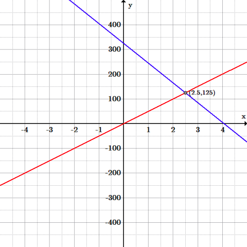 Trains: Train A (red line) is represented by the equation: [latex]y=50x[/latex], and Train B (blue line) is represented by the equation: [latex]y=-80x+325[/latex]. The two trains meet at the intersections point [latex](2.5,125)[/latex], which is after [latex]125[/latex] miles in [latex]2.5[/latex] hours.
Fitting a Curve
Curve fitting with a line attempts to draw a line so that it "best fits" all of the data.Learning Objectives
Use the least squares regression formula to calculate the line of best fit for a set of pointsKey Takeaways
Key Points
- Curve fitting is useful for finding a curve that best fits the data. This allows assumptions about how the data is roughly spread out and predictions about future data points.
- Linear regression attempts to graph a line that best fits the data.
- Ordinary least squares approximation is a type of linear regression that minimizes the sum of the squares of the difference between the approximated value (from the line), and the actual value.
- The slope of the line that approximates [latex]n[/latex] data points is given by [latex]m=\frac{\sum_{i=1}^{n}x_{i}y_{i}-\frac{1}{n}\sum_{i=1}^{n}x_{i}\sum_{j=1}^{n}y_{j}}{\sum_{i=1}^{n}(x_{i}^{2})-\frac{1}{n}(\sum_{i=1}^{n}x_{i})^{2}}[/latex].
- The [latex]y[/latex]-intercept of the line that approximates [latex]n[/latex] data points is given by: [latex]b= \displaystyle{\frac{1}{n} \sum_{i=1}^{n} y_{1} - m \frac{1}{n} \sum_{i=1}^{n} x_{i} = \left (\bar{y} - m \bar{x} \right)} [/latex]
Key Terms
- curve fitting: The process of constructing a curve, or a mathematical function, that has the best fit to a series of data points, possibly subject to constraints.
- outlier: A value in a statistical sample which does not fit a pattern nor describes most other data points.
- least squares approximation: An attempt to minimize the sums of the squared distance between the predicted point and the actual point.
- linear regression: An approach to modeling the linear relationship between a dependent variable, [latex]y[/latex] and an independent variable, [latex]x[/latex].
Curve Fitting
Curve fitting is the process of constructing a curve, or mathematical function, that has the best fit to a series of data points, possibly subject to constraints. Curve fitting can involve either interpolation, where an exact fit to the data is required, or smoothing, in which a "smooth" function is constructed that approximately fits the data. Fitted curves can be used as an aid for data visualization, to infer values of a function where no data are available, and to summarize the relationships among two or more variables. Extrapolation refers to the use of a fitted curve beyond the range of the observed data, and is subject to a greater degree of uncertainty since it may reflect the method used to construct the curve as much as it reflects the observed data. In this section, we will only be fitting lines to data points, but it should be noted that one can fit polynomial functions, circles, piece-wise functions, and any number of functions to data and it is a heavily used topic in statistics.Linear Regression Formula
Linear regression is an approach to modeling the linear relationship between a dependent variable, [latex]y[/latex] and an independent variable, [latex]x[/latex]. With linear regression, a line in slope-intercept form, [latex]y=mx+b[/latex] is found that "best fits" the data. The simplest and perhaps most common linear regression model is the ordinary least squares approximation. This approximation attempts to minimize the sums of the squared distance between the line and every point. [latex]\displaystyle m=\frac{\sum_{i=1}^{n}x_{i}y_{i}-\frac{1}{n}\sum_{i=1}^{n}x_{i}\sum_{j=1}^{n}y_{j}}{\sum_{i=1}^{n}(x_{i}^{2})-\frac{1}{n}(\sum_{i=1}^{n}x_{i})^{2}}[/latex] To find the slope of the line of best fit, calculate in the following steps:- The sum of the product of the [latex]x[/latex] and [latex]y[/latex] coordinates [latex]\sum_{i=1}^{n}x_{i}y_{i}[/latex].
- The sum of the [latex]x[/latex]-coordinates [latex]\sum_{i=1}^{n}x_{i}[/latex].
- The sum of the [latex]y[/latex]-coordinates [latex]\sum_{j=1}^{n}y_{j}[/latex].
- The sum of the squares of the [latex]x[/latex]-coordinates [latex]\sum_{i=1}^{n}(x_{i}^{2})[/latex].
- The sum of the [latex]x[/latex]-coordinates squared [latex](\sum_{i=1}^{n}x_{i})^{2}[/latex].
- The quotient of the numerator and denominator.
- The average of the [latex]y[/latex]-coordinates. Let [latex]\bar{y}[/latex], pronounced [latex]y[/latex]-bar, represent the mean (or average) [latex]y[/latex] value of all the data points: [latex]\bar y =\frac{1}{n}\sum_{i=1}^{n} y_{i}[/latex].
- The average of the [latex]x[/latex]-coordinates. Respectively [latex]\bar{x}[/latex], pronounced [latex]x[/latex]-bar, is the mean (or average) [latex]x[/latex] value of all the data points: [latex]\bar x=\frac{1}{n}\sum_{i=1}^{n} x_{i}[/latex].
- Replace values into the formula above [latex]b=\bar{y} - m \bar{x}[/latex].
Using the Least Squares Approximation
Example: Write the least squares fit line and then graph the line that best fits the data
For [latex]n=8[/latex] points: [latex](-1,0),(0,0),(1,1),(2,2),(3,1),(4,2.5),(5,3) [/latex] and [latex](6,4)[/latex].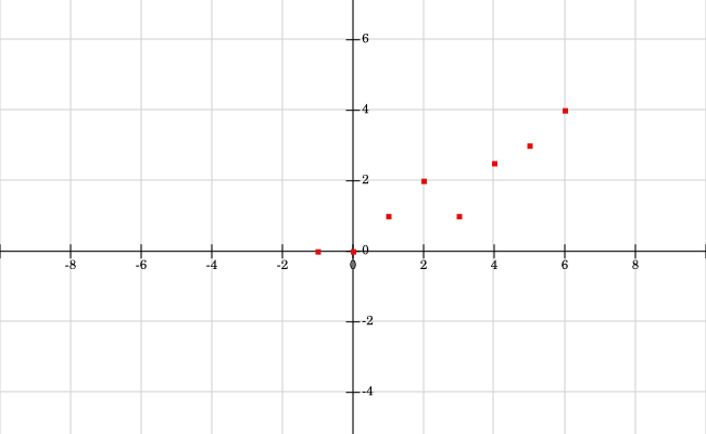 Example Points: The points are graphed in a scatterplot fashion.
First, find the slope [latex](m)[/latex] and [latex]y[/latex]-intercept [latex](b)[/latex] that best approximate this data, using the equations from the prior section:
To find the slope, calculate:- The sum of the product of the [latex]x[/latex] and [latex]y[/latex] coordinates [latex]\sum_{i=1}^{n}x_{i}y_{i}[/latex].
- The sum of the [latex]x[/latex]-coordinates [latex]\sum_{i=1}^{n}x_{i}[/latex].
- The sum of the [latex]y[/latex]-coordinates [latex]\sum_{i=1}^{n}y_{i}[/latex].
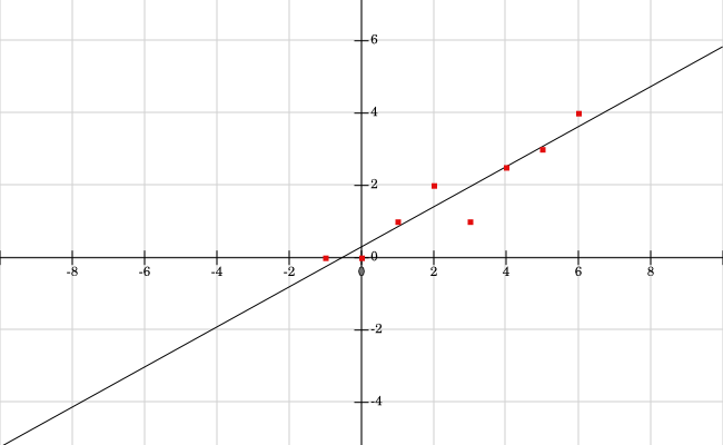 Least Squares Fit Line: The line found by the least squares approximation, [latex]y = 0.554x+0.3025[/latex]. Notice 4 points are above the line, and 4 points are below the line.
Outliers and Least Square Regression
If we have a point that is far away from the approximating line, then it will skew the results and make the line much worse. For instance, let's say in our original example, instead of the point [latex](-1,0)[/latex] we have [latex](-1,6)[/latex]. Using the same calculations as above with the new point, the results are:[latex]m\approx0.0536[/latex] and [latex]b\approx2.3035[/latex], to get the new equation [latex]y=0.0536x+2.3035[/latex]. Looking at the points and line in the new figure below, this new line does not fit the data well, due to the outlier [latex](-1,6)[/latex]. Indeed, trying to fit linear models to data that is quadratic, cubic, or anything non-linear, or data with many outliers or errors can result in bad approximations.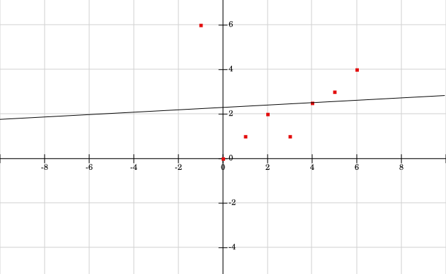 Outlier Approximated Line: Here is the approximated line given the new outlier point at (-1, 6).
Licenses & Attributions
CC licensed content, Shared previously
- Curation and Revision. Authored by: Boundless.com. License: Public Domain: No Known Copyright.
CC licensed content, Specific attribution
- rate of change. Provided by: Wikipedia Located at: https://en.wikipedia.org/wiki/Rate_(mathematics). License: CC BY-SA: Attribution-ShareAlike.
- Algebra/Word Problems. Provided by: Wikibooks License: CC BY-SA: Attribution-ShareAlike.
- slope. Provided by: Wiktionary License: CC BY-SA: Attribution-ShareAlike.
- linear equation. Provided by: Wiktionary License: CC BY-SA: Attribution-ShareAlike.
- Original figure by Julien Coyne. Licensed CC BY-SA 4.0. Provided by: Julien Coyne License: CC BY-SA: Attribution-ShareAlike.
- Mathematical model. Provided by: Wikipedia License: CC BY-SA: Attribution-ShareAlike.
- Boundless. Provided by: Boundless Learning License: CC BY-SA: Attribution-ShareAlike.
- mathematical model. Provided by: Wiktionary License: CC BY-SA: Attribution-ShareAlike.
- Original figure by Julien Coyne. Licensed CC BY-SA 4.0. Provided by: Julien Coyne License: CC BY-SA: Attribution-ShareAlike.
- Original figure by Julien Coyne. Licensed CC BY-SA 4.0. Provided by: Julien Coyne License: CC BY-SA: Attribution-ShareAlike.
- Linear regression. Provided by: Wikipedia License: CC BY-SA: Attribution-ShareAlike.
- Curve fitting. Provided by: Wikipedia License: CC BY-SA: Attribution-ShareAlike.
- Ordinary least squares. Provided by: Wikipedia License: CC BY-SA: Attribution-ShareAlike.
- Boundless. Provided by: Boundless Learning License: CC BY-SA: Attribution-ShareAlike.
- Boundless. Provided by: Boundless Learning License: CC BY-SA: Attribution-ShareAlike.
- outlier. Provided by: Wiktionary Located at: https://en.wiktionary.org/wiki/outlier. License: CC BY-SA: Attribution-ShareAlike.
- Boundless. Provided by: Boundless Learning License: CC BY-SA: Attribution-ShareAlike.
- Original figure by Julien Coyne. Licensed CC BY-SA 4.0. Provided by: Julien Coyne License: CC BY-SA: Attribution-ShareAlike.
- Original figure by Julien Coyne. Licensed CC BY-SA 4.0. Provided by: Julien Coyne License: CC BY-SA: Attribution-ShareAlike.
- FAQ | FooPlot | Online graphing calculator and function plotter. Provided by: Work at Home Jobs Located at: http://fooplot.com/faq. License: Public Domain: No Known Copyright.
- FAQ | FooPlot | Online graphing calculator and function plotter. Provided by: Work at Home Jobs Located at: http://fooplot.com/faq. License: Public Domain: No Known Copyright.
- FAQ | FooPlot | Online graphing calculator and function plotter. Provided by: Work at Home Jobs Located at: http://fooplot.com/faq. License: Public Domain: No Known Copyright.
