
Applications of Quadratic Functions
Scientific Applications of Quadratic Functions
Quadratic relationships between variables are commonly found in physical sciences, engineering, and elsewhere.Learning Objectives
Use the quadratic equation to model phenomena studied in scienceKey Takeaways
Key Points
- The Pythagorean Theorem, [latex]c^2=a^2+b^2[/latex]relates the length of the hypotenuse ([latex]c[/latex]) of a right triangle to the lengths of its legs ([latex]a[/latex] and [latex]b[/latex]).
- Problems involving gravity and projectile motion are typically dependent upon a second-order variable, usually time or initial velocity depending on the relationship.
- Coulomb's Law, which relates electrostatic force, charge amount and distance between two charged particles, has a second-order dependence on the separation of the particles. Solving for either charge results in a quadratic function.
Key Terms
- acceleration: The change of velocity with respect to time (can include changing direction).
- velocity: A vector quantity that denotes the rate of change of position with respect to time, or a speed with the directional component.
The Pythagorean Theorem
The Pythagorean Theorem is used to relate the three sides of right triangles. It states: [latex-display]c^2=a^2+b^2[/latex-display] This says that the square of the length of the hypotenuse ([latex]c[/latex]) is equal to the sum of the squares of the two legs ([latex]a[/latex] and [latex]b[/latex]) of the triangle. This has been proven in many ways, among the most famous of which was devised by Euclid. In practice, the Pythagorean Theorem is often solved via factoring or completing the square. If any of the variables [latex]a[/latex], [latex]b[/latex], or [latex]c[/latex] represent functions in themselves, it is often useful to expand the terms, combine like variables, and then re-factor the expression.Gravity and Projectile Motion
Most all equations involving gravity include a second-order relationship.Gravitational Force
Consider the equation relating gravitational force ([latex]F[/latex]) between two objects to the masses of each object ([latex]m_1[/latex] and [latex]m_2[/latex]) and the distance between them ([latex]r[/latex]): [latex-display]F=G\dfrac {m_1m_2}{r^2}[/latex-display] The shape of this function is not a parabola, but becomes such a shape if rearranged to solve for [latex]m_1[/latex] or [latex]m_2[/latex], as seen below: [latex-display]m_2 = \frac{Fr^2}{Gm_1} = (\frac{F}{Gm_1}) r^2[/latex-display] The general form of this function is: [latex-display]a(x-h)^2 + k[/latex-display] which you should recognize as the vertex form of a quadratic equation.Projectile Motion
The maximum height of a projectile launched directly upwards can also be calculated from a quadratic relationship. The formula relates height ([latex]h[/latex]) to initial velocity ([latex]v_0[/latex]) and gravitational acceleration ([latex]g[/latex]): [latex-display]h=\frac {v_0^2}{2g}[/latex-display] The same maximum height of a projectile launched directly upwards can be found using the time at the projectile's peak ([latex]t_h[/latex]): [latex-display]h=v_0t_h(\frac {1}{2})gt_h^2[/latex-display] Substituting any time ([latex]t[/latex]) in place of [latex]t_h[/latex] leaves the equation for height as a quadratic function of time.Electrostatic Force
The equation relating electrostatic force ([latex]F[/latex]) between two particles, the particles' respective charges ([latex]q_1[/latex] and [latex]q_2[/latex]), and the distance between them ([latex]r[/latex]) is very similar to the aforementioned formula for gravitational force: [latex-display]F=\frac {q_1q_2}{4\pi \epsilon_0r^2}[/latex-display] This is known as Coulomb's Law. Solving for either charge results in a quadratic equation where the charge is dependent on [latex]r^2[/latex].Financial Applications of Quadratic Functions
For problems involving quadratics in finance, it is useful to graph the equation. From these, one can easily find critical values of the function by inspection.Learning Objectives
Apply the quadratic function to real world financial modelsKey Takeaways
Key Points
- In some financial math problems, several key points on a quadratic function are desired, so it can become tedious to calculate each algebraically.
- Rather than calculating each key point of a function, one can find these values by inspection of its graph.
- Graphs of quadratic functions can be used to find key points in many different relationships, from finance to science and beyond.
Example
Consider the function: [latex-display]F(x)=-\frac {x^2}{10}+50x-750[/latex-display] Suppose this models a profit function [latex]f(x)[/latex] in dollars that a company earns as a function of [latex]x[/latex] number of products of a given type that are sold, and is valid for values of [latex]x[/latex] greater than or equal to [latex]0[/latex] and less than or equal to [latex]500[/latex]. If a financier wanted to find the number of sales required to break even, the maximum possible loss (and the number of sales required for this loss), and the maximum profit (and the number of sales required for this profit), they could simply reference a graph instead of calculating it out algebraically.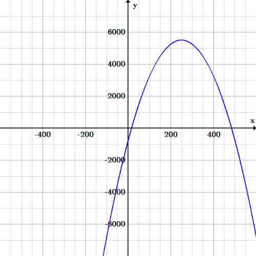 Financial example: Graph of the equation [latex]F(x) = -\frac{x^2}{10} + 50x - 750[/latex], where the x-axis is number of sales, and the y-axis is the monetary return.
Licenses & Attributions
CC licensed content, Shared previously
- Curation and Revision. Authored by: Boundless.com. License: Public Domain: No Known Copyright.
CC licensed content, Specific attribution
- Pythagorean theorem. Provided by: Wikipedia License: CC BY-SA: Attribution-ShareAlike.
- Projectile motion. Provided by: Wikipedia License: CC BY-SA: Attribution-ShareAlike.
- acceleration. Provided by: Wiktionary License: CC BY-SA: Attribution-ShareAlike.
- velocity. Provided by: Wiktionary License: CC BY-SA: Attribution-ShareAlike.
- Quadratic equation. Provided by: Wikipedia License: CC BY-SA: Attribution-ShareAlike.
- Original figure by Julien Coyne. Licensed CC BY-SA 4.0. Provided by: Julien Coyne License: CC BY-SA: Attribution-ShareAlike.
