
Properties of Functions
Increasing, Decreasing, and Constant Functions
Functions can either be constant, increasing as [latex]x[/latex] increases, or decreasing as [latex]x [/latex] increases.Learning Objectives
Apply the definitions of increasing and decreasing functions to determine whether a function is increasing, decreasing, or neither in a given intervalKey Takeaways
Key Points
- A constant function is a function whose values do not vary, regardless of the input into the function.
- An increasing function is one where for every [latex]x_{1}[/latex] and [latex]x_{2}[/latex] that satisfies [latex]x_{2}[/latex]> [latex]x_{1}[/latex], then [latex]f(x_{2}) \geq f(x_{1})[/latex]. If it is strictly greater than, then it is strictly increasing.
- A decreasing function is one where for every [latex]x_{1}[/latex] and [latex]x_{2}[/latex] that satisfies [latex]x_{2}[/latex]> [latex]x_{1}[/latex], then [latex]f(x_{2}) \leq f(x_{1})[/latex]. If it is strictly less than, then it is strictly decreasing.
Key Terms
- decreasing function: Any function of a real variable whose value decreases (or is constant) as the variable increases.
- constant function: A function whose value is the same for all the elements of its domain.
- increasing function: Any function of a real variable whose value increases (or is constant) as the variable increases.
Graphical Behavior of Functions
As part of exploring how functions change, we can identify intervals over which the function is changing in specific ways. We say that a function is increasing on an interval if the function values increase as the input values increase within that interval. Similarly, a function is decreasing on an interval if the function values decrease as the input values increase over that interval.- An increasing function is one where for every [latex]x_1[/latex] and [latex]x_2[/latex] that satisfies [latex]x_2 > x_1[/latex], then [latex]f(x_{2}) \geq f(x_{1})[/latex]. If it is strictly greater than [latex](f(x_2)>f(x_1))[/latex], then it is strictly increasing.
- A decreasing function is one where for every [latex]x_1[/latex]and [latex]x_2[/latex] that satisfies [latex]x_2 > x_1[/latex], then [latex]f(x_{2}) \leq f(x_{1})[/latex]. If it is strictly less than [latex](f(x_2) < f(x_1))[/latex], then it is strictly decreasing.
 Types of Functions: The function [latex]f(x)=x^3−12x[/latex] is increasing on the [latex]x[/latex]-axis from negative infinity to [latex]-2[/latex] and also from [latex]2[/latex] to positive infinity. The interval notation is written as: [latex](−∞, −2)∪(2, ∞)[/latex]. The function is decreasing on on the interval: [latex] (−2, 2)[/latex].
Constant Functions
In mathematics, a constant function is a function whose values do not vary, regardless of the input into the function. A function is a constant function if [latex]f(x)=c[/latex] for all values of [latex]x[/latex] and some constant [latex]c[/latex]. The graph of the constant function [latex]y(x)=c[/latex] is a horizontal line in the plane that passes through the point [latex](0,c).[/latex]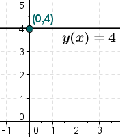 Constant Function: The graph of [latex]f(x)=4 [/latex] illustrates a constant function.
Identifying Function Behavior
Example 1: Identify the intervals where the function is increasing, decreasing, or constant.
Look at the graph from left to right on the [latex]x[/latex]-axis; the first part of the curve is decreasing from infinity to the [latex]x[/latex]-value of [latex]-1[/latex] and then the curve increases. The curve increases on the interval from [latex]-1[/latex] to [latex]1[/latex] and then it decreases again to infinity. Increasing Decreasing Function Graph: For the function pictured above, the curve is decreasing across the intervals: [latex](-\infty,-1)\cup (1,\infty )[/latex] and increasing on the interval [latex] (-1,1)[/latex].
Relative Minima and Maxima
Relative minima and maxima are points of the smallest and greatest values in their neighborhoods respectively.Learning Objectives
Determine the local and global maxima and minima of a given functionKey Takeaways
Key Points
- Minima and maxima are collectively known as extrema.
- A function has a global (or absolute) maximum point at [latex]x[/latex]* if [latex]f(x*) ≥ f(x)[/latex] for all [latex]x[/latex].
- A function has a global (or absolute) minimum point at [latex]x[/latex]* if [latex]f(x*) ≤ f(x)[/latex] for all [latex]x[/latex].
- A function [latex]f[/latex] has a relative (local) maximum at [latex]x=b[/latex] if there exists an interval [latex](a,c)[/latex] with [latex]a<b<c[/latex] such that, for any [latex]x[/latex] in the interval [latex](a,c)[/latex], [latex]f(x)≤f(b)[/latex].
- A function [latex]f[/latex] has a relative (local) minimum at [latex]x=b[/latex] if there exists an interval [latex](a,c)[/latex] with [latex]a<b<c[/latex] such that, for any [latex]x[/latex] in the interval [latex](a,c)[/latex], [latex]f(x)≥f(b)[/latex].
- Functions don't necessarily have extrema in them. For example any line, [latex]f(x) = mx+b[/latex] where [latex]m[/latex] and [latex]b[/latex] are constants, does not have any extrema, be they local or global.
Key Terms
- maximum: The greatest value of a set.
- extremum: A point, or value, which is a maximum or a minimum.
- minimum: The smallest value of a set.
Definitions of Minimums and Maximums: Relative versus Global
In mathematics, the maximum and minimum of a function (known collectively as extrema) are the largest and smallest value that a function takes at a point either within a given neighborhood (local or relative extremum ) or within the function domain in its entirety (global or absolute extremum). Examples of Relative and Global Extrema: This graph has examples of all four possibilities: relative (local) maximum and minimum, and global maximum and minimum.
While some functions are increasing (or decreasing) over their entire domain, many others are not. A value of the input where a function changes from increasing to decreasing (as we go from left to right, that is, as the input variable increases) is called a relative maximum. If a function has more than one, we say it has local maxima. Similarly, a value of the input where a function changes from decreasing to increasing as the input variable increases is called a relative minimum. The plural form is local minima.
A function is also neither increasing nor decreasing at extrema. Note that we have to speak of local extrema, because any given local extremum as defined here is not necessarily the highest maximum or lowest minimum in the function’s entire domain.- A function [latex]f[/latex] has a relative (local) maximum at [latex]x=b[/latex] if there exists an interval [latex](a,c)[/latex] with [latex]a<b<c[/latex] such that, for any [latex]x[/latex] in the interval [latex](a,c)[/latex], [latex]f(x)≤f(b)[/latex].
- Likewise, [latex]f[/latex] has a relative (local) minimum at [latex]x=b[/latex] if there exists an interval [latex](a,c)[/latex] with [latex]a<b<c[/latex] such that, for any [latex]x[/latex] in the interval [latex](a,c)[/latex], [latex]f(x)≥f(b)[/latex].
 Local Maximum Minimum Graph: For the function pictured, the local maximum is at the [latex]y[/latex]-value of 16, and it occurs when [latex]x=-2[/latex]. The local minimum is at the [latex]y[/latex]-value of−16 and it occurs when [latex]x=2[/latex].
A function has a global (or absolute) maximum point at [latex]x[/latex]* if [latex]f(x∗) ≥ f(x)[/latex] for all [latex]x[/latex]. Similarly, a function has a global (or absolute) minimum point at [latex]x[/latex] if [latex]f(x∗) ≤ f(x) [/latex] for all [latex]x[/latex]. Global extrema are also relative extrema.
Functions may not have any extrema in them, such as the line [latex]y=x[/latex]. This line increases towards infinity and decreases towards negative infinity, and has no relative extrema.Distingushing Relative and Global Maximum and Minimum
Example 1: Find all maxima and minima in the graph below:
 Relative Max and Min graph: This curve shows a relative minimum at [latex](-1,-2)[/latex] and relative maximum at [latex](1,2)[/latex].
The graph attains a local maximum at [latex](1,2)[/latex] because it is the highest point in an open interval around [latex]x=1[/latex]. The local maximum is the y-coordinate at [latex]x=1[/latex] which is [latex]2[/latex].
The graph attains a local minimum at [latex](-1,-2)[/latex] because it is the lowest point in an open interval around [latex]x=-1[/latex]. The local minimum is the y-coordinate [latex]x=-1[/latex]which is [latex]-2[/latex].Example 2: Find all global maxima and minima in the graph below:
 Global Max and Min Graph: For the function pictured above, the absolute maximum occurs twice at [latex]y=16[/latex] and the absolute minimum is at [latex](3,-10)[/latex].
The graph attains an absolute maximum in two locations, [latex]x=-2[/latex] and [latex]x=2[/latex], because at these locations, the graph attains its highest point on the domain of the function. The absolute maximum is the y-coordinate which is [latex]16[/latex].
The graph attains an absolute minimum at [latex]x=3[/latex], because it is the lowest point on the domain of the function’s graph. The absolute minimum is the y-coordinate which is [latex]-10[/latex].Piecewise Functions
A piecewise function is defined by multiple subfunctions that are each applied to separate intervals of the inputLearning Objectives
Practice graphing piecewise functions and determine their domains and rangesKey Takeaways
Key Points
- Piecewise functions are defined using the common functional notation, where the body of the function is an array of functions and associated subdomains.
- The absolute value, [latex]\left | x \right |[/latex] is a very common piecewise function. For a real number, its value is [latex]-x[/latex] when [latex]x<0[/latex] and its value is [latex]x[/latex] when [latex]x\geq0[/latex].
- Piecewise functions may have horizontal or vertical gaps (or both) in their functions. A horizontal gap means that the function is not defined for those inputs.
- An open circle at the end of an interval means that the end point is not included in the interval, i.e. strictly less than or strictly greater than. A closed circle means the end point is included.
Key Terms
- subdomain: A domain that is part of a larger domain.
- absolute value: For a real number, its numerical value without regard to its sign; formally, [latex]-1[/latex] times the number if the number is negative, and the number unmodified if it is zero or positive.
- piecewise function: A function in which more than one formula is used to define the output over different pieces of the domain.
Graphing Piecewise Functions
Example 1: Consider the piecewise definition of the absolute value function:
[latex]\displaystyle \left | x \right |= \left\{\begin{matrix} -x, & if\ x<0\\ x, & if\ x\geq0 \end{matrix}\right.[/latex] For all [latex]x[/latex]-values less than zero, the first function [latex](-x)[/latex] is used, which negates the sign of the input value, making the output values positive. Allowing [latex]y=f(x)[/latex], where [latex]f(x)=|x|[/latex], some ordered pair examples of [latex](x,|x|)[/latex] are: [latex]\displaystyle (-2,2) \\ (-1,1) \\ (-0.5,0.5)[/latex] For all values of [latex]x[/latex] greater than or equal to zero, the second function [latex](x)[/latex] is used, making the output values equal to the input values. Some ordered pair examples are: [latex]\displaystyle (2,2) \\ (1,1) \\ (0.5,0.5)[/latex] After finding and plotting some ordered pairs for all parts ("pieces") of the function the result is the V-shaped curve of the absolute value function below. Piecewise function: absolute value: The piecewise function, [latex]\left | x \right |= \left\{\begin{matrix} -x, & if\ x<0\\ x, & if\ x\geq0 \end{matrix}\right.[/latex], is the graph of the absolute value function. Each part of the function is graphed based upon the specific domain chosen.
Example 2: Graph the function and determine its domain and range:
[latex]\displaystyle f(x)= \left\{\begin{matrix} x^2, & if\ x \leq 1\\ 3, & if\ 1 Piecewise Function: The piecewise function [latex]f(x)= \left\{\begin{matrix} x^2, & if\ x \leq 1\\ 3, & if\ 1<x\leq 2\\ x, & if\ x>2\\ \end{matrix}\right.[/latex] has three parts (pieces). Depending on the value of the domain, each piece is different.
Notice the open and closed circles in the graph. This has to do with the specific domains for each part of the function. An open circle at the end of an interval means that the end point is not included in the interval, i.e. strictly less than or strictly greater than. A closed circle means the end point is included (equal to).
The domain of the function starts at negative infinity and continues through each piece, without any gaps, to positive infinity. Since there is an closed AND open dot at [latex]x=1[/latex] the function is piecewise continuous there. When [latex]x=2[/latex], the function is also piecewise continuous. Therefore the domain of this function is the set of all real numbers, [latex]\mathbb{R}[/latex]. The range begins at the lowest [latex]y[/latex]-value, [latex]y=0[/latex] and is continuous through positive infinity. Even though there looks like a gap from [latex]y=1[/latex] to [latex]y=2[/latex], the piece of the function [latex]f(x)=x^2[/latex] includes those values. Therefore the range of the piecewise function is also the set of all real numbers greater than or equal to [latex]0[/latex], or all non-negative values: [latex]y \geq 0[/latex].One-to-One Functions
A one-to-one function, also called an injective function, never maps distinct elements of its domain to the same element of its codomain.Learning Objectives
Use the properties of one-to-one functions to determine if a given function is one-to-oneKey Takeaways
Key Points
- A one-to-one function has a unique output for each unique input.
- Domain restriction can allow a function to become one-to-one, such as in the case of [latex]f(x)=x^2[/latex] for [latex]x\geq 0[/latex].
- To check if a function is a one-to-one perform the horizontal line test. If any horizontal line intersects the graph in more than one point, the function is not one-to-one.
- If every element of a function's range corresponds to exactly one element of its domain, then the function is said to be one-to-one.
Key Terms
- injective function: A function that preserves distinctness: it never maps distinct elements of its domain to the same element of its codomain.
Properties of a One-To-One Function
A one-to-one function, also called an injective function, never maps distinct elements of its domain to the same element of its co-domain. In other words, every element of the function's range corresponds to exactly one element of its domain. Occasionally, an injective function from [latex]X[/latex] to [latex]Y[/latex] is denoted [latex]f: X \mapsto Y[/latex], using an arrow with a barbed tail. An easy way to check if a function is a one-to-one is by graphing it and then performing the horizontal line test. If any horizontal line intersects the graph at more than one point, the function is not one-to-one. To see this, note that the points of intersection have the same y-value, because they lie on the line, but different x values, which by definition means the function cannot be one-to-one.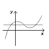 Horizontal line test: Because the horizontal line crosses the graph of the function more than once, it fails the horizontal line test and cannot be one-to-one.
Determining If a Function is One-To-One
Example 1: Is the function [latex]f(x)={x}^{2}[/latex] (with no domain restrictions) one-to-one?
One way to check if the function is one-to-one is to graph the function and perform the horizontal line test. The graph below shows that it forms a parabola and fails the horizontal line test.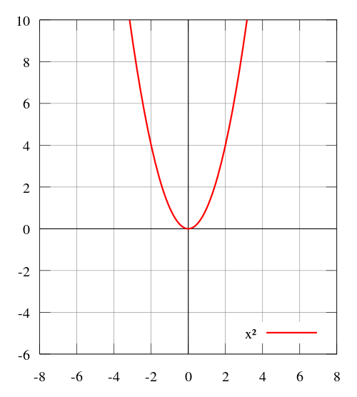
Parabola graph
The graph of the function [latex]f(x)=x^2[/latex] fails the horizontal line test and is therefore not a one-to-one function. If a horizontal line can go through two or more points on the function's graph then the function is not one-to-one. Another way to determine if the function is one-to-one is to make a table of values and check to see if every element of the range corresponds to exactly one element of the domain. A list of ordered pairs for the function are: [latex]\displaystyle (-2,4)\\ (-1,1)\\ (0,0)\\ (1,1)\\ (2,4)[/latex] The ordered pairs [latex](-2,4)[/latex] and [latex](2,4)[/latex] do not pass the definition of one-to-one because the element [latex]4[/latex] of the range corresponds to to [latex]-2[/latex] and [latex]2[/latex]. Each unique input must have a unique output so the function cannot be one-to-one. Notice also, that these two ordered pairs form a horizontal line; which also means that the function is not one-to-one as stated earlier.Example 2: Is the function [latex]f(x)=\left | x \right |[/latex] one-to-one?
This is an absolute value function, which is graphed below. Notice it fails the horizontal line test. Because each unique input does not have a unique output, this function cannot be one-to-one.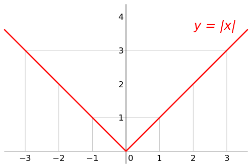 Absolute value graph: The graph of the function,[latex]f(x)=\left | x \right |[/latex], fails the horizontal line test and is therefore not a one-to-one function.
Symmetry of Functions
Two objects have symmetry if one object can be obtained from the other by a transformation.Learning Objectives
Determine whether or not a given relation shows some form of symmetryKey Takeaways
Key Points
- A function has symmetry if it can be transformed in some way without changing the function.
- A function can be symmetric about a point if it can be rotated a fixed amount around that point without changing it.
- A function can be symmetric about a line if it can be reflected over that line without changing it.
Key Terms
- symmetry: A property in mathematics where an object can undergo a transformation while preserving its properties.
Symmetry
In mathematics, an object such as a shape or a function has symmetry if it can be transformed in some way that preserves the properties of the mathematical object. In geometry, a geometric shape or object is symmetric if it can be divided into two or more identical pieces that are arranged in an organized fashion.s means that an object is symmetric if there is a transformation that moves individual pieces of the object but doesn't change the overall shape. For functions, a function exhibits symmetry if each point of a function can be changed according to a mathematical rule without changing the overall function. Determining symmetry can involve graphing the function or evaluating the function algebraically.Symmetric Function Types
Functions and relations can be symmetric about a point, a line, or an axis. They can also have symmetry after a reflection. To determine if a relation has symmetry, graph the relation or function and see if the original curve is a reflection of itself over a point, line, or axis. The image below shows examples of reflecting a function over the [latex]x[/latex]-axis (vertical reflection) and over the [latex]y[/latex]-axis (horizontal reflection). Reflection: A function can be reflected over the [latex]x[/latex] or [latex]y[/latex] axis. If the function looks the same after the reflection, the function is symmetric over that axis.
In the next graph below, quadratic functions have symmetry over a line called the axis of symmetry. The axis splits the U-shaped curve into two parts of the curve which are reflected over the axis of symmetry.
 Symmetry Parabola: The function [latex]y=x^2+4x+3[/latex] shows an axis of symmetry about the line [latex]x=-2[/latex]. The curve is split into [latex]2[/latex] equivalent halves. Notice that the [latex]x[/latex]-intercepts are reflected points over the axis of symmetry and are equidistant from the axis.
Determining Symmetry
Example: Does the function below show symmetry?
 Symmetry about a point: The graph above has symmetry since the points labeled are reflected over the origin.
The graph has symmetry over the origin or point [latex](0,0)[/latex]. The points given, [latex](1,3)[/latex] and [latex](-1,-3)[/latex] are reflected across the origin.
Even and Odd Functions
Functions that have an additive inverse can be classified as odd or even depending on their symmetry properties.Learning Objectives
Determine whether a function is even, odd, or neitherKey Takeaways
Key Points
- The parity of a function does not necessarily reveal whether the function is odd or even.
- Even functions are algebraically defined as functions in which the following relationship holds for all values of: [latex]f(x)=f(-x)[/latex].
- An even function is symmetric about the [latex]y[/latex]-axis: for every point [latex](x,y)[/latex] on the graph, the corresponding point [latex](-x,y)[/latex] or vice versa is also on the graph.
- Odd functions are algebraically defined as functions in which the following relationship holds true for all values of: [latex]-f(x)=f(-x)[/latex].
- An odd function is symmetric with respect to the origin: for every point [latex](x,y)[/latex] on the graph, the corresponding point [latex](-x,-y)[/latex] or vice versa is also on the graph. In other words, rotating the graph [latex]180[/latex] degrees about the point of origin results in the same, unchanged graph.
Key Terms
- parity: A set with the property of having all of its elements belonging to one of two disjoint subsets, especially a set of integers split in subsets of even and odd elements.
- additive inverse: The opposite with respect of addition.
Even and Odd Definitions
Functions can be classified as "odd" or "even" based on their composition. These labels correlate with symmetry properties of the function. The terms "odd" and "even" can only be applied to a limited set of functions. For a function to be classified as one or the other, it must have an additive inverse. Therefore, it must have a number that, when added to it, equals [latex]0[/latex]. Oftentimes, the parity of a function will reveal whether it is odd or even. For example, the function [latex]f(x)=x^2[/latex] is even because it has an exponent, [latex]2[/latex], that is an even integer. This, however, does not apply in every instance. For example, [latex]f(x)=\left | x^3 \right |[/latex] has an exponent that is of an odd integer, [latex]3[/latex], but is also an even function. How can we check if a function is odd or even? Let's look at their characteristics.Even Functions
Even functions are algebraically defined as functions in which the following relationship holds for all values of [latex]x[/latex]: [latex]\displaystyle f(x)=f(-x)[/latex] To check if a function is even, any [latex]x[/latex]-value chosen must yield the same output value when substituted into the function as [latex]-x[/latex].Example 1: Is the function [latex]f(x)=x^4+2x[/latex] even?
Remember the degree of the function, in this case a [latex]4[/latex] which is even, may not always dictate if the function is in fact even. First, perform an algebraic check: Substitute a value for [latex]x[/latex] and [latex]-x[/latex] into the function and check that the same output is found. Let [latex]x=2[/latex]: will [latex]f(2)=f(-2)?[/latex] [latex]\displaystyle \begin{align} f(2)&=(2)^4+2(2)\\ &=16+4\\ &=20 \end{align}[/latex] [latex]\displaystyle \begin{align} f(-2)&=(-2)^4+2(-2)\\ &=16-4\\ &=12 \end{align}[/latex] Therefore [latex]f(2)\neq f(-2)[/latex] and the function is not even.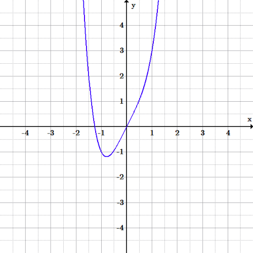 Symmetry: even function?: The function [latex]f(x)=x^4+2x[/latex] pictured above is not even because the graph is not symmetric about the [latex]y[/latex]-axis. For example the point [latex](-1,-1)[/latex] does not reflect onto the point [latex](1,-1)[/latex].
We can confirm this graphically: functions that satisfy the requirements of being even are symmetric about the [latex]y[/latex]-axis. Therefore, for every point [latex](x,y)[/latex] on the graph, the corresponding point [latex](-x,y)[/latex] or vice versa, is also on the graph.
Odd Functions
Odd functions are algebraically defined as functions in which the following relationship holds true for all values of [latex]x[/latex]: [latex]\displaystyle -f(x)=f(-x)[/latex] This relationship can also be expressed as: [latex]\displaystyle f(x)+f(-x)=0[/latex] To check if a function is odd, the negation of the function (be sure to negate all terms of the function) must yield the same output as substituting the value [latex]-x[/latex].Example 2: Is the function [latex]f(x)=x^3-9x[/latex] odd?
Algebraic check: Does [latex]-f(x)=f(-x)[/latex]? [latex]\displaystyle \begin{align} -f(x)&=-(x^3-9x)\\& =-x^3+9x \end{align}[/latex] [latex]\displaystyle \begin{align} f(-x)&=(-x)^3-9(-x)\\& =-x^3+9x \end{align}[/latex] Therefore [latex]-f(x)=f(-x)[/latex] and the function is odd. Graphical check: Functions that satisfy the requirements of being odd are symmetric with respect to the origin. In other words, rotating the graph [latex]180[/latex] degrees about the point of origin results in the same, unchanged graph. In addition, for every point [latex](x,y)[/latex] on the graph, the corresponding point [latex](-x,-y)[/latex] is also on the graph.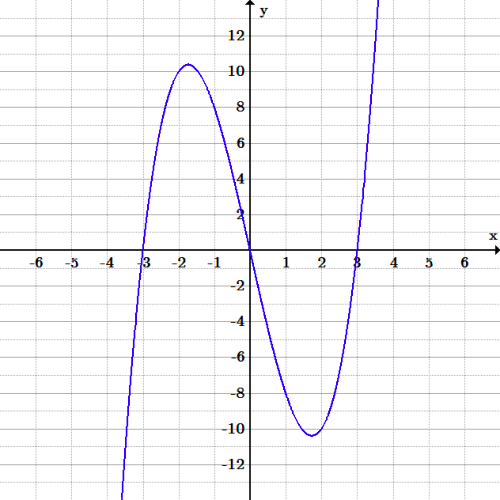 Symmetry: odd function?: The function, [latex]f(x)=x^3-9x[/latex] is odd since the graph is symmetric about the origin. One can also check that any point is symmetric about the origin: for example, does [latex](-1,8)[/latex] yield [latex](1,-8)[/latex]? Yes, those two points are symmetric about the origin.
Licenses & Attributions
CC licensed content, Shared previously
- Curation and Revision. Authored by: Boundless.com. License: Public Domain: No Known Copyright.
CC licensed content, Specific attribution
- decreasing function. Provided by: Wiktionary License: CC BY-SA: Attribution-ShareAlike.
- Constant function. Provided by: Wikipedia License: CC BY-SA: Attribution-ShareAlike.
- increasing function. Provided by: Wiktionary License: CC BY-SA: Attribution-ShareAlike.
- constant function. Provided by: Wiktionary License: CC BY-SA: Attribution-ShareAlike.
- Increasing Decreasing Function Graph.jpg. Provided by: Openstax Located at: https://openstax.org/books/college-algebra/pages/3-3-rates-of-change-and-behavior-of-graphs. License: CC BY-SA: Attribution-ShareAlike.
- Constant Function. Provided by: Wikipedia Located at: https://en.wikipedia.org/wiki/Constant_function#/media/File:Wiki_constant_function_175_200.png. License: CC BY-SA: Attribution-ShareAlike.
- Types of Function. Provided by: Open Stax Located at: https://openstax.org/books/college-algebra/pages/3-3-rates-of-change-and-behavior-of-graphs. License: CC BY-SA: Attribution-ShareAlike.
- maximum and minimum. Provided by: Openstax License: CC BY-SA: Attribution-ShareAlike.
- Maxima and minima. Provided by: Wikipedia License: CC BY-SA: Attribution-ShareAlike.
- Boundless. Provided by: Boundless Learning License: CC BY-SA: Attribution-ShareAlike.
- maximum. Provided by: Wiktionary Located at: https://en.wiktionary.org/wiki/maximum. License: CC BY-SA: Attribution-ShareAlike.
- extremum. Provided by: Wiktionary License: CC BY-SA: Attribution-ShareAlike.
- Increasing Decreasing Function Graph.jpg. Provided by: Openstax Located at: https://openstax.org/books/college-algebra/pages/3-3-rates-of-change-and-behavior-of-graphs. License: CC BY-SA: Attribution-ShareAlike.
- Constant Function. Provided by: Wikipedia License: CC BY-SA: Attribution-ShareAlike.
- Types of Function. Provided by: Open Stax Located at: https://openstax.org/books/college-algebra/pages/3-3-rates-of-change-and-behavior-of-graphs. License: CC BY-SA: Attribution-ShareAlike.
- Extrema example original. Provided by: Wikipedia License: Public Domain: No Known Copyright.
- Global max and min Graph. Provided by: Openstax Located at: https://openstax.org/books/college-algebra/pages/3-3-rates-of-change-and-behavior-of-graphs. License: CC BY-SA: Attribution-ShareAlike.
- Relative Max and Min Graph. Provided by: Openstax License: CC BY-SA: Attribution-ShareAlike.
- Max Min Graph. Provided by: Openstax Located at: https://openstax.org/books/college-algebra/pages/3-3-rates-of-change-and-behavior-of-graphs. License: CC BY-SA: Attribution-ShareAlike.
- Piecewise functions. Provided by: Wikipedia Located at: https://en.wikipedia.org/wiki/Piecewise_functions. License: CC BY-SA: Attribution-ShareAlike.
- Algebra/Functions. Provided by: Wikibooks License: CC BY-SA: Attribution-ShareAlike.
- subdomain. Provided by: Wiktionary License: CC BY-SA: Attribution-ShareAlike.
- Boundless. Provided by: Boundless Learning License: CC BY-SA: Attribution-ShareAlike.
- absolute value. Provided by: Wiktionary License: CC BY-SA: Attribution-ShareAlike.
- Increasing Decreasing Function Graph.jpg. Provided by: Openstax Located at: https://openstax.org/books/college-algebra/pages/3-3-rates-of-change-and-behavior-of-graphs. License: CC BY-SA: Attribution-ShareAlike.
- Constant Function. Provided by: Wikipedia Located at: https://en.wikipedia.org/wiki/Constant_function#/media/File:Wiki_constant_function_175_200.png. License: CC BY-SA: Attribution-ShareAlike.
- Types of Function. Provided by: Open Stax Located at: https://openstax.org/books/college-algebra/pages/3-3-rates-of-change-and-behavior-of-graphs. License: CC BY-SA: Attribution-ShareAlike.
- Extrema example original. Provided by: Wikipedia License: Public Domain: No Known Copyright.
- Global max and min Graph. Provided by: Openstax Located at: https://openstax.org/books/college-algebra/pages/3-3-rates-of-change-and-behavior-of-graphs. License: CC BY-SA: Attribution-ShareAlike.
- Relative Max and Min Graph. Provided by: Openstax License: CC BY-SA: Attribution-ShareAlike.
- Max Min Graph. Provided by: Openstax Located at: https://openstax.org/books/college-algebra/pages/3-3-rates-of-change-and-behavior-of-graphs. License: CC BY-SA: Attribution-ShareAlike.
- Absolute_value.png. Provided by: Wikimedia Commons License: CC BY-SA: Attribution-ShareAlike.
- Graphing Piecewise Function. Provided by: Openstax Located at: https://openstax.org/books/college-algebra/pages/3-2-domain-and-range. License: CC BY-SA: Attribution-ShareAlike.
- One-to-one function. Provided by: Wikipedia License: CC BY-SA: Attribution-ShareAlike.
- Horizontal line test. Provided by: Wikipedia License: CC BY-SA: Attribution-ShareAlike.
- injective function. Provided by: Wikipedia License: CC BY-SA: Attribution-ShareAlike.
- Increasing Decreasing Function Graph.jpg. Provided by: Openstax Located at: https://openstax.org/books/college-algebra/pages/3-3-rates-of-change-and-behavior-of-graphs. License: CC BY-SA: Attribution-ShareAlike.
- Constant Function. Provided by: Wikipedia Located at: https://en.wikipedia.org/wiki/Constant_function#/media/File:Wiki_constant_function_175_200.png. License: CC BY-SA: Attribution-ShareAlike.
- Types of Function. Provided by: Open Stax Located at: https://openstax.org/books/college-algebra/pages/3-3-rates-of-change-and-behavior-of-graphs. License: CC BY-SA: Attribution-ShareAlike.
- Extrema example original. Provided by: Wikipedia License: Public Domain: No Known Copyright.
- Global max and min Graph. Provided by: Openstax Located at: https://openstax.org/books/college-algebra/pages/3-3-rates-of-change-and-behavior-of-graphs. License: CC BY-SA: Attribution-ShareAlike.
- Relative Max and Min Graph. Provided by: Openstax License: CC BY-SA: Attribution-ShareAlike.
- Max Min Graph. Provided by: Openstax Located at: https://openstax.org/books/college-algebra/pages/3-3-rates-of-change-and-behavior-of-graphs. License: CC BY-SA: Attribution-ShareAlike.
- Absolute_value.png. Provided by: Wikimedia Commons License: CC BY-SA: Attribution-ShareAlike.
- Graphing Piecewise Function. Provided by: Openstax Located at: https://openstax.org/books/college-algebra/pages/3-2-domain-and-range. License: CC BY-SA: Attribution-ShareAlike.
- Absolute_value.png. Provided by: Wikimedia commons Located at: https://commons.wikimedia.org/wiki/File:Absolute_value.svg. License: CC BY-SA: Attribution-ShareAlike.
- Horizontal-test-fail.png. Provided by: Wikipedia Located at: https://upload.wikimedia.org/wikipedia/commons/f/f9/Horizontal-test-fail.png?uselang=en-ca. License: CC BY-SA: Attribution-ShareAlike.
- 500px-Function_x^2.svg.png. Provided by: Wikimedia Commons License: CC BY-SA: Attribution-ShareAlike.
- Symmetry in math. Provided by: Openstax Located at: https://openstax.org/books/algebra-and-trigonometry/pages/5-2-power-functions-and-polynomial-functions. License: CC BY-SA: Attribution-ShareAlike.
- Symmetry in mathematics. Provided by: Wikipedia License: CC BY-SA: Attribution-ShareAlike.
- Symmetry in mathematics. Provided by: Wikipedia License: CC BY-SA: Attribution-ShareAlike.
- Increasing Decreasing Function Graph.jpg. Provided by: Openstax Located at: https://openstax.org/books/college-algebra/pages/3-3-rates-of-change-and-behavior-of-graphs. License: CC BY-SA: Attribution-ShareAlike.
- Constant Function. Provided by: Wikipedia Located at: https://en.wikipedia.org/wiki/Constant_function#/media/File:Wiki_constant_function_175_200.png. License: CC BY-SA: Attribution-ShareAlike.
- Types of Function. Provided by: Open Stax Located at: https://openstax.org/books/college-algebra/pages/3-3-rates-of-change-and-behavior-of-graphs. License: CC BY-SA: Attribution-ShareAlike.
- Extrema example original. Provided by: Wikipedia License: Public Domain: No Known Copyright.
- Global max and min Graph. Provided by: Openstax Located at: https://openstax.org/books/college-algebra/pages/3-3-rates-of-change-and-behavior-of-graphs. License: CC BY-SA: Attribution-ShareAlike.
- Relative Max and Min Graph. Provided by: Openstax License: CC BY-SA: Attribution-ShareAlike.
- Max Min Graph. Provided by: Openstax Located at: https://openstax.org/books/college-algebra/pages/3-3-rates-of-change-and-behavior-of-graphs. License: CC BY-SA: Attribution-ShareAlike.
- Absolute_value.png. Provided by: Wikimedia Commons License: CC BY-SA: Attribution-ShareAlike.
- Graphing Piecewise Function. Provided by: Openstax Located at: https://openstax.org/books/college-algebra/pages/3-2-domain-and-range. License: CC BY-SA: Attribution-ShareAlike.
- Absolute_value.png. Provided by: Wikimedia commons License: CC BY-SA: Attribution-ShareAlike.
- Horizontal-test-fail.png. Provided by: Wikipedia Located at: https://upload.wikimedia.org/wikipedia/commons/f/f9/Horizontal-test-fail.png?uselang=en-ca. License: CC BY-SA: Attribution-ShareAlike.
- 500px-Function_x^2.svg.png. Provided by: Wikimedia Commons Located at: https://commons.wikimedia.org/wiki/File:Function_x%5E2.svg. License: CC BY-SA: Attribution-ShareAlike.
- Reflection Image.jpg. Provided by: Openstax Located at: https://openstax.org/books/algebra-and-trigonometry/pages/3-5-transformation-of-functions. License: CC BY-SA: Attribution-ShareAlike.
- Symmetry Parabola.jpg. Provided by: Openstax License: CC BY-SA: Attribution-ShareAlike.
- odd function symmetry.jpg. Provided by: Openstax Located at: https://openstax.org/books/algebra-and-trigonometry/pages/3-5-transformation-of-functions. License: CC BY-SA: Attribution-ShareAlike.
- Openstax. Provided by: even and odd functions License: CC BY-SA: Attribution-ShareAlike.
- Even and odd functions. Provided by: Wikipedia License: CC BY-SA: Attribution-ShareAlike.
- parity. Provided by: Wiktionary License: CC BY-SA: Attribution-ShareAlike.
- additive inverse. Provided by: Wiktionary License: CC BY-SA: Attribution-ShareAlike.
- Increasing Decreasing Function Graph.jpg. Provided by: Openstax Located at: https://openstax.org/books/college-algebra/pages/3-3-rates-of-change-and-behavior-of-graphs. License: CC BY-SA: Attribution-ShareAlike.
- Constant Function. Provided by: Wikipedia License: CC BY-SA: Attribution-ShareAlike.
- Types of Function. Provided by: Open Stax Located at: https://openstax.org/books/college-algebra/pages/3-3-rates-of-change-and-behavior-of-graphs. License: CC BY-SA: Attribution-ShareAlike.
- Extrema example original. Provided by: Wikipedia License: Public Domain: No Known Copyright.
- Global max and min Graph. Provided by: Openstax Located at: https://openstax.org/books/college-algebra/pages/3-3-rates-of-change-and-behavior-of-graphs. License: CC BY-SA: Attribution-ShareAlike.
- Relative Max and Min Graph. Provided by: Openstax License: CC BY-SA: Attribution-ShareAlike.
- Max Min Graph. Provided by: Openstax Located at: https://openstax.org/books/college-algebra/pages/3-3-rates-of-change-and-behavior-of-graphs. License: CC BY-SA: Attribution-ShareAlike.
- Absolute_value.png. Provided by: Wikimedia Commons Located at: https://commons.wikimedia.org/wiki/File:Absolute_value.svg. License: CC BY-SA: Attribution-ShareAlike.
- Graphing Piecewise Function. Provided by: Openstax Located at: https://openstax.org/books/college-algebra/pages/3-2-domain-and-range. License: CC BY-SA: Attribution-ShareAlike.
- Absolute_value.png. Provided by: Wikimedia commons License: CC BY-SA: Attribution-ShareAlike.
- Horizontal-test-fail.png. Provided by: Wikipedia Located at: https://upload.wikimedia.org/wikipedia/commons/f/f9/Horizontal-test-fail.png?uselang=en-ca. License: CC BY-SA: Attribution-ShareAlike.
- 500px-Function_x^2.svg.png. Provided by: Wikimedia Commons License: CC BY-SA: Attribution-ShareAlike.
- Reflection Image.jpg. Provided by: Openstax Located at: https://openstax.org/books/algebra-and-trigonometry/pages/3-5-transformation-of-functions. License: CC BY-SA: Attribution-ShareAlike.
- Symmetry Parabola.jpg. Provided by: Openstax License: CC BY-SA: Attribution-ShareAlike.
- odd function symmetry.jpg. Provided by: Openstax Located at: https://openstax.org/books/algebra-and-trigonometry/pages/3-5-transformation-of-functions. License: CC BY-SA: Attribution-ShareAlike.
- Original figure by Julien Coyne. Licensed CC BY-SA 4.0. Provided by: Julien Coyne License: CC BY-SA: Attribution-ShareAlike.
- Original figure by Julien Coyne. Licensed CC BY-SA 4.0. Provided by: Julien Coyne License: CC BY-SA: Attribution-ShareAlike.
