
Precalculus Review
Real Numbers, Functions, and Graphs
Functions relate a set of inputs to a set of outputs such that each input is related to exactly one output. Graphs can be used to represent these relationships pictorially.Learning Objectives
Generate a function, sketch a graphKey Takeaways
Key Points
- The real numbers include all the rational numbers, such as the integer −5 and the fraction [latex]\displaystyle \frac{4}{3}[/latex], and all the irrational numbers such as [latex]\sqrt{2}[/latex] (1.41421356… the square root of two, an irrational algebraic number) and [latex]\pi[/latex] (3.14159265…, a transcendental number).
- A function is a relation between a set of inputs and a set of permissible outputs with the property that each input is related to exactly one output.
- The graph of a function f is the collection of all ordered pairs [latex](x, f(x))[/latex].
Key Terms
- domain: the set of all possible mathematical entities (points) where a given function is defined
- Cartesian: of or pertaining to coordinates based on mutually orthogonal axes
Real Numbers
Real numbers can be thought of as points on an infinitely long line called the number line or real line, where the points corresponding to integers are equally spaced. The real numbers include all the rational numbers, such as the integer -5 and the fraction [latex]\displaystyle \frac{4}{3}[/latex], and all the irrational numbers such as [latex]\sqrt{2}[/latex] (1.41421356… the square root of two, an irrational algebraic number) and [latex]\pi[/latex] (3.14159265…, a transcendental number). Any real number can be determined by a possibly infinite decimal representation such as that of 8.632, where each consecutive digit is measured in units one tenth the size of the previous one. The real line can be thought of as a part of the complex plane, and correspondingly, complex numbers include real numbers as a special case.Functions
A function is a relation between a set of inputs and a set of permissible outputs with the property that each input is related to exactly one output. An example is the function that relates each real number [latex]x[/latex] to its square: [latex]f(x)= x^{2}[/latex]. Here, the domain is the entire set of real numbers and the function maps each real number to its square. The output of a function [latex]f[/latex] corresponding to an input [latex]x[/latex] is denoted by [latex]f(x)[/latex](read "f of x"). In this example, if the input is [latex]-3[/latex], then the output is 9, and we may write [latex]f(-3) = 9[/latex]. The input variable(s) are sometimes referred to as the argument(s) of the function.Graphs
The graph of a function [latex]f[/latex] is the collection of all ordered pairs [latex](x, f(x))[/latex]. In particular, if [latex]x[/latex] is a real number, "graph" means the graphical representation of this collection, in the form of a line chart, a curve on a Cartesian plane, together with Cartesian axes, etc. Graphing on a Cartesian plane is sometimes referred to as curve sketching. If the function input [latex]x[/latex] is an ordered pair [latex](x_1, x_2)[/latex] of real numbers, the graph is the collection of all ordered triples [latex](x_1, x_2, f(x_1, x_2))[/latex] and its graphical representation is a surface (see the three-dimensional graph below).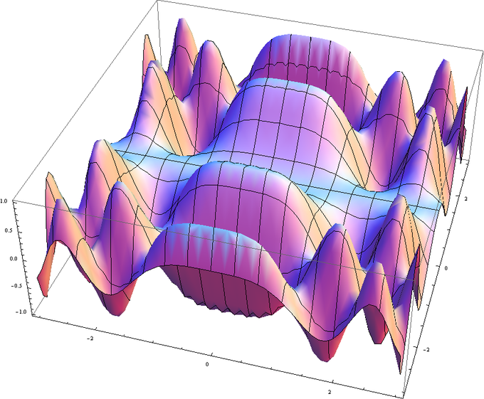
Graph of a Function: This is a graph of the function [latex]f(x,y) = \sin{x^2} \cos{y^2}[/latex]
Linear and Quadratic Functions
Linear and quadratic functions make lines and a parabola, respectively, when graphed and are some of the simplest functional forms.Learning Objectives
Identify linear and quadratic functionsKey Takeaways
Key Points
- Linear function refers to a function that satisfies the following two linearity properties: [latex]f(x + y) = f(x) + f(y) \\ f(ax) = af(x).[/latex]
- Linear functions may be confused with affine functions. One variable affine functions can be written as [latex]f(x)=mx+b[/latex], which makes a line when graphed.
- A quadratic function, in mathematics, is a polynomial function of the form: [latex]f(x)=ax^2+bx+c,\quad a \ne 0[/latex]. The graph of a quadratic function is a parabola whose axis of symmetry is parallel to the y-axis.
Key Terms
- polynomial: an expression consisting of a sum of a finite number of terms, each term being the product of a constant coefficient and one or more variables raised to a non-negative integer power
- linearity: a relationship between several quantities which can be considered proportional and expressed in terms of linear algebra; any mathematical property of a relationship, operation, or function that is analogous to such proportionality, satisfying additivity and homogeneity
Linear Function
In calculus and algebra, the term linear function refers to a function that satisfies the following two linearity properties: [latex-display]f(x + y) = f(x) + f(y) \\ f(ax) = af(x)[/latex-display] Linear functions may be confused with affine functions. One variable affine functions can be written as [latex]f(x)=mx+b[/latex]. Although affine functions make lines when graphed, they do not satisfy the properties of linearity. However, the term "linear function" is quite often loosely used to include affine functions of the form [latex]f(x)=mx+b[/latex]. Linear functions form the basis of linear algebra.Affine Function
An affine transformation (from the Latin, affinis, "connected with") is a transformation which preserves straight lines (i.e., all points lying on a line initially still lie on a line after transformation) and ratios of distances between points lying on a straight line (e.g., the midpoint of a line segment remains the midpoint after transformation). It does not necessarily preserve angles or lengths, but does have the property that sets of parallel lines will remain parallel to each other after an affine transformation.Quadratic Function
A quadratic function, in mathematics, is a polynomial function of the form: [latex]f(x)=ax^2+bx+c, a \ne 0[/latex]. The graph of a quadratic function is a parabola whose axis of symmetry is parallel to the y-axis. The expression [latex]ax^2+bx+c[/latex] in the definition of a quadratic function is a polynomial of degree 2 or second order, or a 2nd degree polynomial, because the highest exponent of [latex]x[/latex] is 2. If the quadratic function is set equal to zero, then the result is a quadratic equation. The solutions to the equation are called the roots of the equation.Trigonometric Functions
Trigonometric functions are functions of an angle, relating the angles of a triangle to the lengths of the sides of a triangle.Learning Objectives
Define the three most familiar trigonometric functionsKey Takeaways
Key Points
- The most familiar trigonometric functions are the sine, cosine, and tangent.
- The sine of an angle is the ratio of the length of the opposite side to the length of the hypotenuse.
- The cosine of an angle is the ratio of the length of the adjacent side to the length of the hypotenuse.
- The tangent of an angle is the ratio of the length of the opposite side to the length of the adjacent side.
Key Terms
- hypotenuse: the side of a right triangle opposite the right angle
- differential equation: an equation involving the derivatives of a function

Sine, Tangent, and Secant: The sine, tangent, and secant functions of an angle constructed geometrically in terms of a unit circle. The number θ is the length of the curve; thus angles are being measured in radians.

Base of Trigonometry: If two right triangles have equal acute angles, they are similar, so their side lengths are proportional. Proportionality constants are written within the image: [latex]\sin{\theta}[/latex], [latex]\cos{\theta}[/latex], [latex]\tan{\theta}[/latex] where [latex]\theta[/latex] is the common measure of five acute angles.
Right-angle Triangle Definitions
The sine of an angle is the ratio of the length of the opposite side to the length of the hypotenuse. In our case [latex]\sin A = \frac {\textrm{opposite}} {\textrm{hypotenuse}} = \frac {a} {h}[/latex]. Note that this ratio does not depend on size of the particular right triangle chosen, as long as it contains the angle [latex]A[/latex], since all such triangles are similar.
Right-Angle Triangle: Right-angle triangle used in defining trigonometric functions.
Inverse Functions
An inverse function is a function that undoes another function: For a function [latex]f(x)=y[/latex] the inverse function, if it exists, is given as [latex]g(y)= x[/latex].Learning Objectives
Compute an inverse functionKey Takeaways
Key Points
- A function [latex]f[/latex] that has an inverse is called invertible; the inverse function is then uniquely determined by [latex]f[/latex] and is denoted by [latex]f^{-1}[/latex].
- If [latex]f[/latex] is invertible, the function [latex]g[/latex] is unique.
- The function [latex]f(x)=x^{2}[/latex] may or may not be invertible, depending on the domain. For a domain containing all real numbers, it is not invertible. But if the domain consists of the non-negative numbers, then the function is injective and invertible.
Key Terms
- domain: the set of all possible mathematical entities (points) where a given function is defined
- injective: of, relating to, or being an injection: such that each element of the image (or range) is associated with at most one element of the preimage (or domain); inverse-deterministic
- range: the set of values (points) which a function can obtain
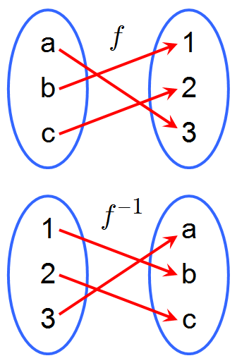
A Function and its Inverse: A function [latex]f[/latex] and its inverse [latex]f^{-1}[/latex]. Because [latex]f[/latex] maps [latex]a[/latex] to 3, the inverse [latex]f^{-1}[/latex] maps 3 back to [latex]a[/latex].
Examples
Inverse operations that lead to inverse functions
Inverse operations are the opposite of direct variation functions. Direct variation function are based on multiplication; [latex]y=kx[/latex]. The opposite operation of multiplication is division and an inverse variation function is [latex]\displaystyle y=\frac{k}{x}[/latex].Squaring and square root functions
The function [latex]f(x)=x^2[/latex] may or may not be invertible, depending on the domain. If the domain is the real numbers, then each element in the range [latex]Y[/latex] would correspond to two different elements in the domain [latex]X[/latex] ([latex]\pm x[/latex]), and therefore [latex]f[/latex] would not be invertible. More precisely, the square of [latex]x[/latex] is not invertible because it is impossible to deduce from its output the sign of its input. Such a function is called non-injective or information-losing. Notice that neither the square root nor the principal square root function is the inverse of [latex]x^2[/latex] because the first is not single-valued, and the second returns [latex]-x[/latex] when [latex]x[/latex] is negative. If the domain consists of the non-negative numbers, then the function is injective and invertible.Exponential and Logarithmic Functions
Both exponential and logarithmic functions are widely used in scientific and engineering applications.Learning Objectives
Compute using logarithmic and exponential functionsKey Takeaways
Key Points
- Exponential function is the function [latex]e^x[/latex], where [latex]e[/latex] is the number (approximately 2.718281828) such that the function [latex]e^x[/latex] is its own derivative.
- The exponential function may be defined by the following power series: [latex]\displaystyle e^x = \sum_{n = 0}^{\infty} \frac{x^n}{n!} = 1 + x + {\frac{x^2}{2!} } + {\frac{x^3}{3!} } + \cdots[/latex].
- The logarithm of a number [latex]x[/latex] with respect to base [latex]b[/latex] is the exponent by which [latex]b[/latex] must be raised to yield [latex]x[/latex]. In other words, the logarithm of [latex]x[/latex] to base [latex]b[/latex] is the solution [latex]y[/latex] to the equation [latex]b^y=x[/latex].
Key Terms
- inverse function: a function that does exactly the opposite of another
- derivative: a measure of how a function changes as its input changes
- binary: the bijective base-2 numeral system, which uses only the digits 0 and 1
Exponential Function
Exponential function is the function [latex]e^x[/latex] the number (approximately 2.718281828) such that the function [latex]e^x[/latex] is its own derivative. The function is often written as [latex]\exp{(x)}[/latex], especially when it is impractical to write the independent variable as a superscript. The exponential function is widely used in physics, chemistry, engineering, mathematical biology, economics and mathematics. Sometimes the term exponential function is used more generally for functions of the form [latex]f(x)=cb^x[/latex], where the base [latex]b[/latex] is any positive real number and [latex]c[/latex] is a constant.
Graph of [latex]f(x)=e^x[/latex]: The derivative (or slope of a tangential line) of the exponential function is equal to the value of the function.
Logarithmic Functions
The logarithm of a number [latex]x[/latex] with respect to base [latex]b[/latex] is the exponent by which [latex]b[/latex] must be raised to yield [latex]x[/latex]. In other words, the logarithm of [latex]x[/latex] to base [latex]b[/latex] is the solution [latex]y[/latex] to the equation [latex]b^y = x[/latex]. For example, the logarithm of 1000 to base 10 is 3, because 1000 is 10 to the power 3: [latex]1000=10\cdot 10 \cdot 10 = 10^3[/latex]. More generally, if [latex]x=b^y[/latex], then [latex]y[/latex] is the logarithm of [latex]x[/latex] to base [latex]b[/latex], and is written [latex]y=\log_b(x)[/latex], so [latex]\log_{10}(1000)=3[/latex].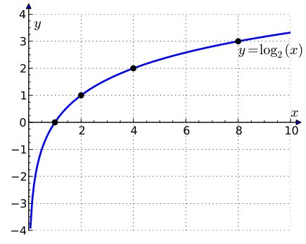
Plot of [latex]\log_2(x)[/latex]: The graph of the logarithm to base 2 crosses the x-axis (horizontal axis) at 1 and passes through the points with coordinates [latex](2,1)[/latex], [latex](4,2)[/latex], and [latex](8,3)[/latex]. For example, [latex]\log_2(8)=3[/latex], because [latex]2^3=8[/latex]. The graph gets arbitrarily close to the y-axis, but does not meet or intersect it.
Using Calculators and Computers
For numerical calculations and graphing, scientific calculators and personal computers are commonly used in classes and laboratories.Learning Objectives
Describe how calculators and computers can assist with arithmetic, graphing, and other complicated operations.Key Takeaways
Key Points
- A scientific calculator is a type of electronic calculator, usually but not always handheld, designed to calculate problems in science, engineering, and mathematics.
- These days, scientific and graphing calculators are often replaced by personal computers or even by supercomputers.
- Either by using commercial softwares or by using programming languages, complicated, multi-step numerical calculations can be performed on a PC.
Key Terms
- supercomputer: any computer that has a far greater processing power than others of its day; typically they use more than one core and are housed in large clean rooms with high air flow to permit cooling. Typical uses are weather forecasting, nuclear simulations and animations
- programming language: code of reserved words and symbols used in computer programs, which give instructions to the computer on how to accomplish certain computing tasks
Scientific calculators
A scientific calculator is a type of electronic calculator, usually but not always handheld, designed to calculate problems in science, engineering, and mathematics. They have almost completely replaced slide rules in almost all traditional applications, and are widely used in both education and professional settings. In certain contexts such as higher education, scientific calculators have been superseded by graphing calculators, which offer a superset of scientific calculator functionality along with the ability to graph input data and write and store programs for the device. There is also some overlap with the financial calculator market.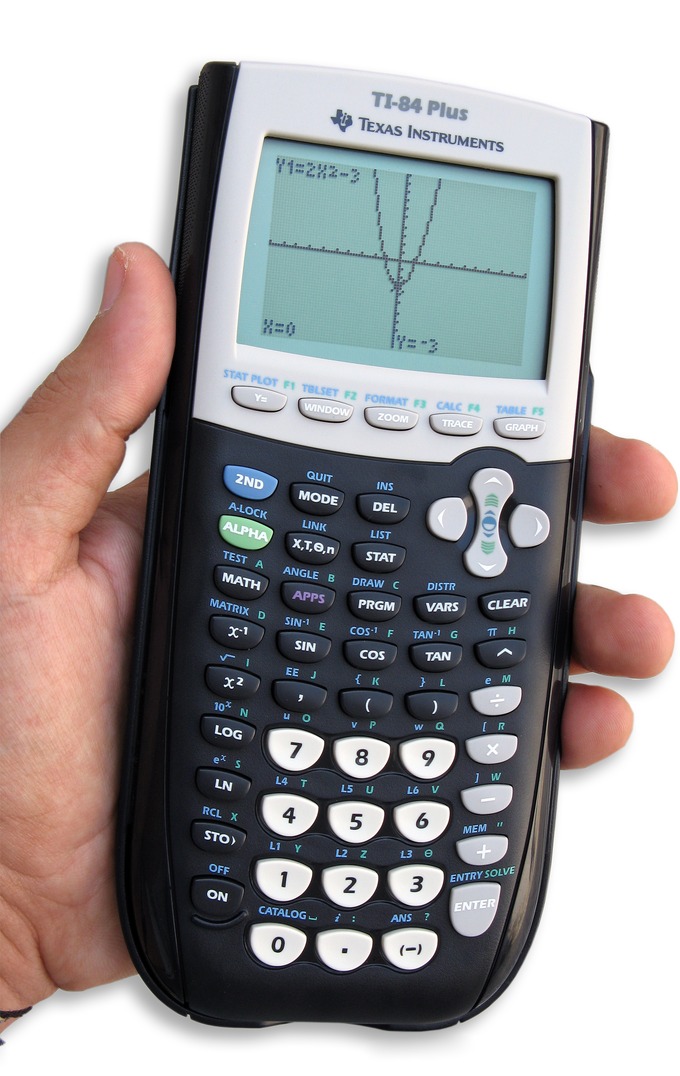
Fig 1: A typical graphing calculator built by Texas Instruments, displaying a graph of a function [latex]f(x)=2x^2-3[/latex].
Computers
These days, scientific and graphing calculators are often replaced by personal computers or even by supercomputers. There are many softwares (such as Mathematica, Matlab, etc.) that allows not only numerical calculations and plotting of functions, but also helping with matrix manipulations, data manipulation, implementation of algorithms, creation of user interfaces, etc. In addition, by using programming languages such as Fortran, C, C++, Java, etc., complicated, multi-step numerical calculations can be performed on a PC. Therefore, computers are extremely useful tools in scientific and engineering disciplines.
Fig 2: A three-dimentional wireframe plot of the unnormalized sinc function [latex]x=\text{sinc}(x^2+y^2)^{\frac{1}{2}}[/latex].
Licenses & Attributions
CC licensed content, Shared previously
- Curation and Revision. Provided by: Boundless.com License: CC BY-SA: Attribution-ShareAlike.
CC licensed content, Specific attribution
- Real number. Provided by: Wikipedia Located at: https://en.wikipedia.org/wiki/Real_number. License: CC BY-SA: Attribution-ShareAlike.
- Graph of a function. Provided by: Wikipedia Located at: https://en.wikipedia.org/wiki/Graph_of_a_function. License: CC BY-SA: Attribution-ShareAlike.
- Function (mathematics). Provided by: Wikipedia Located at: https://en.wikipedia.org/wiki/Function_(mathematics). License: CC BY-SA: Attribution-ShareAlike.
- domain. Provided by: Wiktionary Located at: https://en.wiktionary.org/wiki/domain. License: CC BY-SA: Attribution-ShareAlike.
- Cartesian. Provided by: Wiktionary Located at: https://en.wiktionary.org/wiki/Cartesian. License: CC BY-SA: Attribution-ShareAlike.
- Function (mathematics). Provided by: Wikipedia Located at: https://en.wikipedia.org/wiki/Function_(mathematics). License: CC BY: Attribution.
- Affine function. Provided by: Wikipedia Located at: https://en.wikipedia.org/wiki/Affine_function. License: CC BY-SA: Attribution-ShareAlike.
- Linear function. Provided by: Wikipedia Located at: https://en.wikipedia.org/wiki/Linear_function. License: CC BY-SA: Attribution-ShareAlike.
- Quadratic function. Provided by: Wikipedia Located at: https://en.wikipedia.org/wiki/Quadratic_function. License: CC BY-SA: Attribution-ShareAlike.
- linearity. Provided by: Wiktionary Located at: https://en.wiktionary.org/wiki/linearity. License: CC BY-SA: Attribution-ShareAlike.
- polynomial. Provided by: Wiktionary License: CC BY-SA: Attribution-ShareAlike.
- Function (mathematics). Provided by: Wikipedia License: CC BY: Attribution.
- Trigonometric functions. Provided by: Wikipedia License: CC BY-SA: Attribution-ShareAlike.
- hypotenuse. Provided by: Wiktionary License: CC BY-SA: Attribution-ShareAlike.
- differential equation. Provided by: Wiktionary License: CC BY-SA: Attribution-ShareAlike.
- Function (mathematics). Provided by: Wikipedia License: CC BY: Attribution.
- Trigonometric functions. Provided by: Wikipedia License: CC BY: Attribution.
- Trigonometric functions. Provided by: Wikipedia License: CC BY: Attribution.
- Trigonometric functions. Provided by: Wikipedia License: CC BY: Attribution.
- Inverse function. Provided by: Wikipedia License: CC BY-SA: Attribution-ShareAlike.
- injective. Provided by: Wiktionary License: CC BY-SA: Attribution-ShareAlike.
- domain. Provided by: Wiktionary License: CC BY-SA: Attribution-ShareAlike.
- range. Provided by: Wiktionary License: CC BY-SA: Attribution-ShareAlike.
- Function (mathematics). Provided by: Wikipedia License: CC BY: Attribution.
- Trigonometric functions. Provided by: Wikipedia License: CC BY: Attribution.
- Trigonometric functions. Provided by: Wikipedia License: CC BY: Attribution.
- Trigonometric functions. Provided by: Wikipedia License: CC BY: Attribution.
- Inverse function. Provided by: Wikipedia License: CC BY: Attribution.
- Exponential function. Provided by: Wikipedia License: CC BY-SA: Attribution-ShareAlike.
- Logarithm. Provided by: Wikipedia License: CC BY-SA: Attribution-ShareAlike.
- derivative. Provided by: Wikipedia License: CC BY-SA: Attribution-ShareAlike.
- binary. Provided by: Wiktionary License: CC BY-SA: Attribution-ShareAlike.
- inverse function. Provided by: Wiktionary License: CC BY-SA: Attribution-ShareAlike.
- Function (mathematics). Provided by: Wikipedia License: CC BY: Attribution.
- Trigonometric functions. Provided by: Wikipedia License: CC BY: Attribution.
- Trigonometric functions. Provided by: Wikipedia License: CC BY: Attribution.
- Trigonometric functions. Provided by: Wikipedia License: CC BY: Attribution.
- Inverse function. Provided by: Wikipedia License: CC BY: Attribution.
- Exponential function. Provided by: Wikipedia License: CC BY: Attribution.
- Binary_logarithm_plot_with_ticks.png. Provided by: Wikipedia License: CC BY-SA: Attribution-ShareAlike.
- Scientific calculator. Provided by: Wikipedia License: CC BY-SA: Attribution-ShareAlike.
- supercomputer. Provided by: Wiktionary License: CC BY-SA: Attribution-ShareAlike.
- programming language. Provided by: Wiktionary License: CC BY-SA: Attribution-ShareAlike.
- Function (mathematics). Provided by: Wikipedia License: CC BY: Attribution.
- Trigonometric functions. Provided by: Wikipedia License: CC BY: Attribution.
- Trigonometric functions. Provided by: Wikipedia License: CC BY: Attribution.
- Trigonometric functions. Provided by: Wikipedia Located at: https://en.wikipedia.org/wiki/Trigonometric_functions. License: CC BY: Attribution.
- Inverse function. Provided by: Wikipedia License: CC BY: Attribution.
- Exponential function. Provided by: Wikipedia License: CC BY: Attribution.
- Binary_logarithm_plot_with_ticks.png. Provided by: Wikipedia License: CC BY-SA: Attribution-ShareAlike.
- Scientific calculator. Provided by: Wikipedia License: CC BY: Attribution.
- Matlab. Provided by: Wikipedia License: CC BY: Attribution.
