
Putting It Together
The model we saw at the beginning is a logistic growth model. The equation for this specific model is: [latex-display]{P}=\frac{{100}}{{{1}+{50}^{-0.5x}}}[/latex-display] Again, P is measured in millions of dollars of sales and x is measured in thousands of dollars of advertising. Q1 We can actually graph this function and we know that the derivative of this function measures the rate of change. In this case, we can calculate the derivative and find its value at x = 2, or if we did not have the equation, we can use our table / graph and get an estimate for the derivative between the points x = 2 and x = 3 (i.e. use the average rate of change between these points to estimate the instantaneous rate of change at x = 2). Q2 We should note that there is a horizontal asymptote which this function never crosses (i.e. there is a point where we simply will not sell any more of this item regardless of the amount of money we spend on advertising. There is also a point where change in sales stops increasing and start decreasing based on the advertising dollar. This is equivalent to a point of concavity on this graph. The point of concavity in this function actually lies at the half-way point on the height of this graph (i.e. at 50 million in sales). If all we had was the data, we would be able to determine when our sales started to “slow down” and then we could actually predict the maximum number of sales. This would allow us to determine when to stop pumping money into the advertising budget.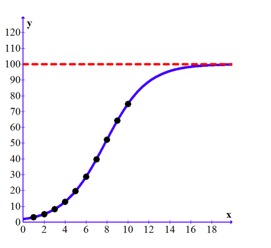
Licenses & Attributions
CC licensed content, Original
- Instantaneous Rate of Change of a Function. Provided by: Columbia Basin College Authored by: Paul Jones. License: CC BY: Attribution.
