
End Behavior of Power Functions
Learning Outcomes
- Identify a power function.
- Describe the end behavior of a power function given its equation or graph.
 Three birds on a cliff with the sun rising in the background. Functions discussed in this module can be used to model populations of various animals, including birds. (credit: Jason Bay, Flickr)
| Year | 2009 | 2010 | 2011 | 2012 | 2013 |
| Bird Population | 800 | 897 | 992 | 1,083 | 1,169 |
Identifying Power Functions
In order to better understand the bird problem, we need to understand a specific type of function. A power function is a function with a single term that is the product of a real number, coefficient, and variable raised to a fixed real number power. Keep in mind a number that multiplies a variable raised to an exponent is known as a coefficient. As an example, consider functions for area or volume. The function for the area of a circle with radius [latex]r[/latex] is:[latex]A\left(r\right)=\pi {r}^{2}[/latex]
and the function for the volume of a sphere with radius r is:[latex]V\left(r\right)=\frac{4}{3}\pi {r}^{3}[/latex]
Both of these are examples of power functions because they consist of a coefficient, [latex]\pi [/latex] or [latex]\frac{4}{3}\pi [/latex], multiplied by a variable r raised to a power.A General Note: Power FunctionS
A power function is a function that can be represented in the form[latex]f\left(x\right)=a{x}^{n}[/latex]
where a and n are real numbers and a is known as the coefficient.Q & A
Is [latex]f\left(x\right)={2}^{x}[/latex] a power function? No. A power function contains a variable base raised to a fixed power. This function has a constant base raised to a variable power. This is called an exponential function, not a power function.tip for success
Unlike a polynomial function, in which all the variable powers must be non-negative integers, a power function only requires the power on the exponent be a real number.Example: Identifying Power Functions
Which of the following functions are power functions?[latex]\begin{array}{c}f\left(x\right)=1\hfill & \text{Constant function}\hfill \\ f\left(x\right)=x\hfill & \text{Identity function}\hfill \\ f\left(x\right)={x}^{2}\hfill & \text{Quadratic}\text{ }\text{ function}\hfill \\ f\left(x\right)={x}^{3}\hfill & \text{Cubic function}\hfill \\ f\left(x\right)=\frac{1}{x} \hfill & \text{Reciprocal function}\hfill \\ f\left(x\right)=\frac{1}{{x}^{2}}\hfill & \text{Reciprocal squared function}\hfill \\ f\left(x\right)=\sqrt{x}\hfill & \text{Square root function}\hfill \\ f\left(x\right)=\sqrt[3]{x}\hfill & \text{Cube root function}\hfill \end{array}[/latex]
Answer: All of the listed functions are power functions. The constant and identity functions are power functions because they can be written as [latex]f\left(x\right)={x}^{0}[/latex] and [latex]f\left(x\right)={x}^{1}[/latex] respectively. The quadratic and cubic functions are power functions with whole number powers [latex]f\left(x\right)={x}^{2}[/latex] and [latex]f\left(x\right)={x}^{3}[/latex]. The reciprocal and reciprocal squared functions are power functions with negative whole number powers because they can be written as [latex]f\left(x\right)={x}^{-1}[/latex] and [latex]f\left(x\right)={x}^{-2}[/latex]. The square and cube root functions are power functions with fractional powers because they can be written as [latex]f\left(x\right)={x}^{1/2}[/latex] or [latex]f\left(x\right)={x}^{1/3}[/latex].
Try It
Which functions are power functions?[latex]\begin{array}{c}f\left(x\right)=2{x}^{2}\cdot 4{x}^{3}\hfill \\ g\left(x\right)=-{x}^{5}+5{x}^{3}-4x\hfill \\ h\left(x\right)=\frac{2{x}^{5}-1}{3{x}^{2}+4}\hfill \end{array}[/latex]
Answer: [latex]f\left(x\right)[/latex] is a power function because it can be written as [latex]f\left(x\right)=8{x}^{5}[/latex]. The other functions are not power functions.
Identifying End Behavior of Power Functions
The graph below shows the graphs of [latex]f\left(x\right)={x}^{2},g\left(x\right)={x}^{4}[/latex], [latex]h\left(x\right)={x}^{6}[/latex], [latex]k(x)=x^{8}[/latex], and [latex]p(x)=x^{10}[/latex] which are all power functions with even, whole-number powers. Notice that these graphs have similar shapes, very much like that of the quadratic function. However, as the power increases, the graphs flatten somewhat near the origin and become steeper away from the origin.
 To describe the behavior as numbers become larger and larger, we use the idea of infinity. We use the symbol [latex]\infty[/latex] for positive infinity and [latex]-\infty[/latex] for negative infinity. When we say that "x approaches infinity," which can be symbolically written as [latex]x\to \infty[/latex], we are describing a behavior; we are saying that x is increasing without bound.
With even-powered power functions, as the input increases or decreases without bound, the output values become very large, positive numbers. Equivalently, we could describe this behavior by saying that as [latex]x[/latex] approaches positive or negative infinity, the [latex]f\left(x\right)[/latex] values increase without bound. In symbolic form, we could write
To describe the behavior as numbers become larger and larger, we use the idea of infinity. We use the symbol [latex]\infty[/latex] for positive infinity and [latex]-\infty[/latex] for negative infinity. When we say that "x approaches infinity," which can be symbolically written as [latex]x\to \infty[/latex], we are describing a behavior; we are saying that x is increasing without bound.
With even-powered power functions, as the input increases or decreases without bound, the output values become very large, positive numbers. Equivalently, we could describe this behavior by saying that as [latex]x[/latex] approaches positive or negative infinity, the [latex]f\left(x\right)[/latex] values increase without bound. In symbolic form, we could write
[latex]\text{as }x\to \pm \infty , f\left(x\right)\to \infty[/latex]
The graph below shows [latex]f\left(x\right)={x}^{3},g\left(x\right)={x}^{5},h\left(x\right)={x}^{7},k\left(x\right)={x}^{9},\text{and }p\left(x\right)={x}^{11}[/latex], which are all power functions with odd, whole-number powers. Notice that these graphs look similar to the cubic function. As the power increases, the graphs flatten near the origin and become steeper away from the origin.
 These examples illustrate that functions of the form [latex]f\left(x\right)={x}^{n}[/latex] reveal symmetry of one kind or another. First, in the even-powered power functions, we see that even functions of the form [latex]f\left(x\right)={x}^{n}\text{, }n\text{ even,}[/latex] are symmetric about the y-axis. In the odd-powered power functions, we see that odd functions of the form [latex]f\left(x\right)={x}^{n}\text{, }n\text{ odd,}[/latex] are symmetric about the origin.
For these odd power functions, as x approaches negative infinity, [latex]f\left(x\right)[/latex] decreases without bound. As x approaches positive infinity, [latex]f\left(x\right)[/latex] increases without bound. In symbolic form we write
These examples illustrate that functions of the form [latex]f\left(x\right)={x}^{n}[/latex] reveal symmetry of one kind or another. First, in the even-powered power functions, we see that even functions of the form [latex]f\left(x\right)={x}^{n}\text{, }n\text{ even,}[/latex] are symmetric about the y-axis. In the odd-powered power functions, we see that odd functions of the form [latex]f\left(x\right)={x}^{n}\text{, }n\text{ odd,}[/latex] are symmetric about the origin.
For these odd power functions, as x approaches negative infinity, [latex]f\left(x\right)[/latex] decreases without bound. As x approaches positive infinity, [latex]f\left(x\right)[/latex] increases without bound. In symbolic form we write
[latex]\begin{array}{c}\text{as } x\to -\infty , f\left(x\right)\to -\infty \\ \text{as } x\to \infty , f\left(x\right)\to \infty \end{array}[/latex]
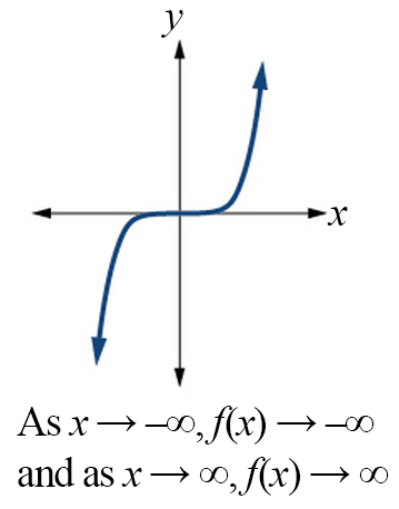
The behavior of the graph of a function as the input values get very small ( [latex]x\to -\infty[/latex] ) and get very large ( [latex]x\to \infty[/latex] ) is referred to as the end behavior of the function. We can use words or symbols to describe end behavior. The table below shows the end behavior of power functions of the form [latex]f\left(x\right)=a{x}^{n}[/latex] where [latex]n[/latex] is a non-negative integer depending on the power and the constant.| Even power | Odd power | |
|---|---|---|
| Positive constanta > 0 | 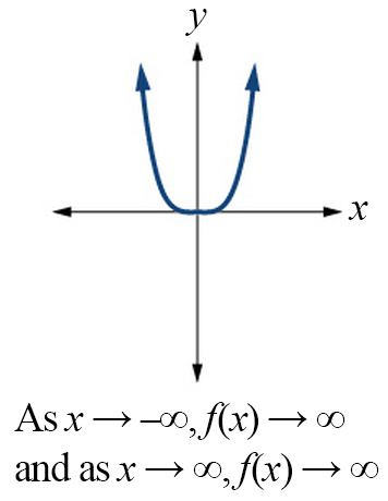 |
 |
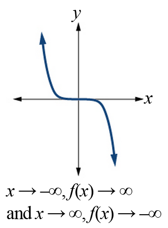
| Negative constanta < 0 | 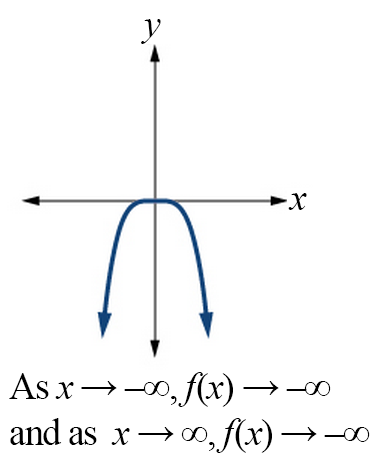 |
 |
How To: Given a power function [latex]f\left(x\right)=a{x}^{n}[/latex] where [latex]n[/latex] is a non-negative integer, identify the end behavior.
- Determine whether the power is even or odd.
- Determine whether the constant is positive or negative.
- Use the above graphs to identify the end behavior.
Example: Identifying the End Behavior of a Power Function
Describe the end behavior of the graph of [latex]f\left(x\right)={x}^{8}[/latex].Answer:
The coefficient is 1 (positive) and the exponent of the power function is 8 (an even number). As x (input) approaches infinity, [latex]f\left(x\right)[/latex] (output) increases without bound. We write as [latex]x\to \infty , f\left(x\right)\to \infty [/latex]. As x approaches negative infinity, the output increases without bound. In symbolic form, as [latex]x\to -\infty , f\left(x\right)\to \infty[/latex]. We can graphically represent the function.

Example: Identifying the End Behavior of a Power Function
Describe the end behavior of the graph of [latex]f\left(x\right)=-{x}^{9}[/latex].Answer:
The exponent of the power function is 9 (an odd number). Because the coefficient is –1 (negative), the graph is the reflection about the x-axis of the graph of [latex]f\left(x\right)={x}^{9}[/latex]. The graph shows that as x approaches infinity, the output decreases without bound. As x approaches negative infinity, the output increases without bound. In symbolic form, we would write as [latex]x\to -\infty , f\left(x\right)\to \infty[/latex] and as [latex]x\to \infty , f\left(x\right)\to -\infty[/latex].

Analysis of the Solution
We can check our work by using the table feature on an online graphing calculator.- Enter the function [latex]f\left(x\right)=-{x}^{9}[/latex] into an online graphing calculator
- Create a table with the following x values, and observe the sign of the outputs. [latex]-10,-5,0,5,10[/latex]
- Now, enter the function [latex]g\left(x\right)={x}^{9}[/latex], and create a similar table. Compare the signs of the outputs for both functions.
Try It
Describe in words and symbols the end behavior of [latex]f\left(x\right)=-5{x}^{4}[/latex].Answer: As x approaches positive or negative infinity, [latex]f\left(x\right)[/latex] decreases without bound: as [latex]x\to \pm \infty , f\left(x\right)\to -\infty[/latex] because of the negative coefficient.
[ohm_question]69337[/ohm_question] [ohm_question]15940[/ohm_question]Licenses & Attributions
CC licensed content, Original
- Revision and Adaptation. Provided by: Lumen Learning License: CC BY: Attribution.
- Even Power Functions Interactive. Authored by: Lumen Learning. Located at: https://www.desmos.com/calculator/rgdspbzldy. License: Public Domain: No Known Copyright.
- Odd Power Functions Interactive. Authored by: Lumen Learning. Located at: https://www.desmos.com/calculator/4aeczmnp1w. License: Public Domain: No Known Copyright.
CC licensed content, Shared previously
- College Algebra. Provided by: OpenStax Authored by: Abramson, Jay et al.. Located at: https://openstax.org/books/college-algebra/pages/1-introduction-to-prerequisites. License: CC BY: Attribution. License terms: Download for free at http://cnx.org/contents/[email protected].
- Question ID 69337. Authored by: Shahbazian, Roy. License: CC BY: Attribution. License terms: IMathAS Community License CC-BY + GPL.
- Question ID 15940. Authored by: Sousa, James. License: CC BY: Attribution. License terms: IMathAS Community License CC-BY + GPL.
- Ex: End Behavior or Long Run Behavior of Functions. Authored by: James Sousa (Mathispower4u.com) . License: CC BY: Attribution.
