
Stretching, Compressing, or Reflecting a Logarithmic Function
Learning Outcomes
- Graph stretches and compressions of logarithmic functions.
- Graph reflections of logarithmic functions.
Graphing Stretches and Compressions of [latex]y=\text{log}_{b}\left(x\right)[/latex]
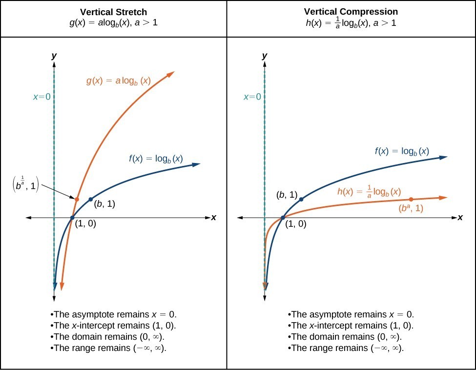
When the parent function [latex]f\left(x\right)={\mathrm{log}}_{b}\left(x\right)[/latex] is multiplied by a constant a > 0, the result is a vertical stretch or compression of the original graph. To visualize stretches and compressions, we set a > 1 and observe the general graph of the parent function [latex]f\left(x\right)={\mathrm{log}}_{b}\left(x\right)[/latex] alongside the vertical stretch, [latex]g\left(x\right)=a{\mathrm{log}}_{b}\left(x\right)[/latex], and the vertical compression, [latex]h\left(x\right)=\frac{1}{a}{\mathrm{log}}_{b}\left(x\right)[/latex].try it
Using an online graphing calculator plot the functions [latex]g(x) = a\log_{b}{x}[/latex] and [latex]h(x) = \frac{1}{a}\log_{b}{x}[/latex]. One represents a vertical compression of the other. You may select any value for [latex]b[/latex], though one between [latex]2[/latex] and [latex]5[/latex] will be easier to see. Experiment with various [latex]a[/latex] values between [latex]1[/latex] and [latex]10[/latex]. As you investigate, consider the following questions:- Both the vertical stretch and compression produce graphs that are increasing. Which transformation produces a function that increases faster?
- One of the key points that is commonly defined for transformations of a logarithmic function comes from finding the input that gives an output of [latex]y = 1[/latex]. This point can help you determine whether a graph is the result of a vertical compression or stretch. Explain why.
A General Note: Vertical Stretches and Compressions of the Parent Function [latex]y=\text{log}_{b}\left(x\right)[/latex]
For any constant a > 1, the function [latex]f\left(x\right)=a{\mathrm{log}}_{b}\left(x\right)[/latex]- stretches the parent function [latex]y={\mathrm{log}}_{b}\left(x\right)[/latex] vertically by a factor of a if a > 1.
- compresses the parent function [latex]y={\mathrm{log}}_{b}\left(x\right)[/latex] vertically by a factor of a if 0 < a < 1.
- has the vertical asymptote x = 0.
- has the x-intercept [latex]\left(1,0\right)[/latex].
- has domain [latex]\left(0,\infty \right)[/latex].
- has range [latex]\left(-\infty ,\infty \right)[/latex].
How To: Given a logarithmic function Of the form [latex]f\left(x\right)=a{\mathrm{log}}_{b}\left(x\right)[/latex], [latex]a>0[/latex], graph the Stretch or Compression
- Identify the vertical stretch or compression:
- If [latex]|a|>1[/latex], the graph of [latex]f\left(x\right)={\mathrm{log}}_{b}\left(x\right)[/latex] is stretched by a factor of a units.
- If [latex]|a|<1[/latex], the graph of [latex]f\left(x\right)={\mathrm{log}}_{b}\left(x\right)[/latex] is compressed by a factor of a units.
- Draw the vertical asymptote x = 0.
- Identify three key points from the parent function. Find new coordinates for the shifted functions by multiplying the y coordinates in each point by a.
- Label the three points.
- The domain is [latex]\left(0,\infty \right)[/latex], the range is [latex]\left(-\infty ,\infty \right)[/latex], and the vertical asymptote is x = 0.
tip for success
Logarithm functions follow the same principles as the other toolkit functions with regard to stretches, compressions, and reflections.Example: Graphing a Stretch or Compression of the Parent Function [latex]y=\text{log}_{b}\left(x\right)[/latex]
Sketch the graph of [latex]f\left(x\right)=2{\mathrm{log}}_{4}\left(x\right)[/latex] alongside its parent function. Include the key points and asymptote on the graph. State the domain, range, and asymptote.Answer: Since the function is [latex]f\left(x\right)=2{\mathrm{log}}_{4}\left(x\right)[/latex], we will note that = 2. This means we will stretch the function [latex]f\left(x\right)={\mathrm{log}}_{4}\left(x\right)[/latex] by a factor of 2. The vertical asymptote is x = 0. Consider the three key points from the parent function, [latex]\left(\frac{1}{4},-1\right)[/latex], [latex]\left(1,0\right)[/latex], and [latex]\left(4,1\right)[/latex]. The new coordinates are found by multiplying the y coordinates of each point by 2. Label the points [latex]\left(\frac{1}{4},-2\right)[/latex], [latex]\left(1,0\right)[/latex], and [latex]\left(4,\text{2}\right)[/latex].
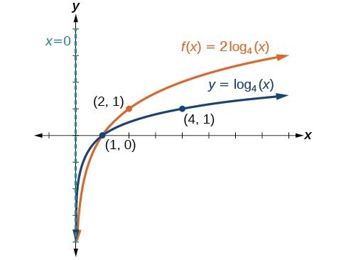 The domain is [latex]\left(0,\infty \right)[/latex], the range is [latex]\left(-\infty ,\infty \right)[/latex], and the vertical asymptote is x = 0.
Try It
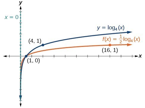
Sketch a graph of [latex]f\left(x\right)=\frac{1}{2}{\mathrm{log}}_{4}\left(x\right)[/latex] alongside its parent function. Include the key points and asymptote on the graph. State the domain, range, and asymptote.Answer:
The domain is [latex]\left(0,\infty \right)[/latex], the range is [latex]\left(-\infty ,\infty \right)[/latex], and the vertical asymptote is x = 0.
Example: Combining a Shift and a Stretch
Sketch the graph of [latex]f\left(x\right)=5\mathrm{log}\left(x+2\right)[/latex]. State the domain, range, and asymptote.Answer: Remember, what happens inside parentheses happens first. First, we move the graph left 2 units and then stretch the function vertically by a factor of 5. The vertical asymptote will be shifted to x = –2. The x-intercept will be [latex]\left(-1,0\right)[/latex]. The domain will be [latex]\left(-2,\infty \right)[/latex]. Two points will help give the shape of the graph: [latex]\left(-1,0\right)[/latex] and [latex]\left(8,5\right)[/latex]. We chose x = 8 as the x-coordinate of one point to graph because when x = 8, x + 2 = 10, the base of the common logarithm.
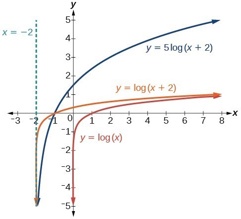 The domain is [latex]\left(-2,\infty \right)[/latex], the range is [latex]\left(-\infty ,\infty \right)[/latex], and the vertical asymptote is x = –2.
Try It
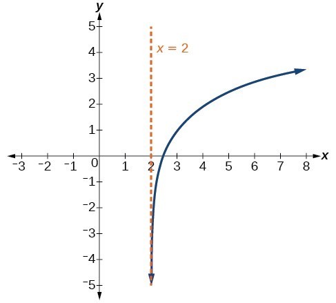
Sketch a graph of the function [latex]f\left(x\right)=3\mathrm{log}\left(x - 2\right)+1[/latex]. State the domain, range, and asymptote.Answer:
The domain is [latex]\left(2,\infty \right)[/latex], the range is [latex]\left(-\infty ,\infty \right)[/latex], and the vertical asymptote is x = 2.
Graphing Reflections of [latex]f\left(x\right)={\mathrm{log}}_{b}\left(x\right)[/latex]
When the parent function [latex]f\left(x\right)={\mathrm{log}}_{b}\left(x\right)[/latex] is multiplied by –1, the result is a reflection about the x-axis. When the input is multiplied by –1, the result is a reflection about the y-axis. To visualize reflections, we restrict b > 1 and observe the general graph of the parent function [latex]f\left(x\right)={\mathrm{log}}_{b}\left(x\right)[/latex] alongside the reflection about the x-axis, [latex]g\left(x\right)={\mathrm{-log}}_{b}\left(x\right)[/latex], and the reflection about the y-axis, [latex]h\left(x\right)={\mathrm{log}}_{b}\left(-x\right)[/latex].Try it
Using an online graphing calculator, plot the functions [latex]f(x) = \log_{b}{x},\text{ }g(x)=-\log_{b}{x},\text{ and }h(x) = \log_{b}({-x}) [/latex]. You may select any value for [latex]b[/latex], though one between [latex]2[/latex] and [latex]5[/latex] will be easier to see. Also plot the point [latex](b,1)[/latex]. Consider the following questions:- Which graph, [latex]g(x) = -\log_{b}{x} \text{ or }h(x) = \log_{b}({-x})[/latex] represents a vertical reflection? Which one represents a horizontal reflection?
- You already added the point [latex](b,1)[/latex] as a point of interest for the function [latex]f(x)[/latex]. Using the variable [latex]b[/latex] as your [latex]x[/latex] value, add the corresponding points of interest for [latex]g(x)\text{ and }h(x)[/latex].
- Does the vertical asymptote change when you reflect the graph of [latex]f(x)[/latex] either vertically or horizontally?
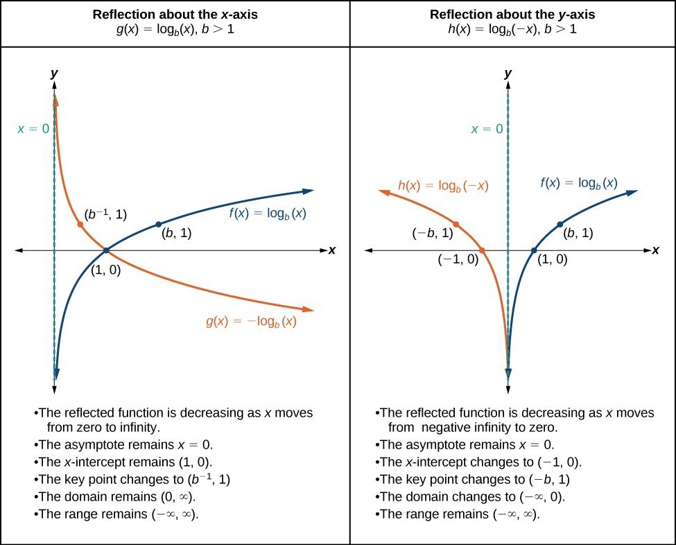
A General Note: Reflections of the Parent Function [latex]y=\text{log}_{b}\left(x\right)[/latex]
The function [latex]f\left(x\right)={\mathrm{-log}}_{b}\left(x\right)[/latex]- reflects the parent function [latex]y={\mathrm{log}}_{b}\left(x\right)[/latex] about the x-axis.
- has domain [latex]\left(0,\infty \right)[/latex], range, [latex]\left(-\infty ,\infty \right)[/latex], and vertical asymptote x = 0 which are unchanged from the parent function.
- reflects the parent function [latex]y={\mathrm{log}}_{b}\left(x\right)[/latex] about the y-axis.
- has domain [latex]\left(-\infty ,0\right)[/latex].
- has range [latex]\left(-\infty ,\infty \right)[/latex] and vertical asymptote x = 0 which are unchanged from the parent function.
How To: Given a logarithmic function with the parent function [latex]f\left(x\right)={\mathrm{log}}_{b}\left(x\right)[/latex], graph a Reflection
| [latex]\text{If }f\left(x\right)=-{\mathrm{log}}_{b}\left(x\right)[/latex] | [latex]\text{If }f\left(x\right)={\mathrm{log}}_{b}\left(-x\right)[/latex] |
|---|---|
| 1. Draw the vertical asymptote, x = 0. | 1. Draw the vertical asymptote, x = 0. |
| 2. Plot the x-intercept, [latex]\left(1,0\right)[/latex]. | 2. Plot the x-intercept, [latex]\left(1,0\right)[/latex]. |
| 3. Reflect the graph of the parent function [latex]f\left(x\right)={\mathrm{log}}_{b}\left(x\right)[/latex] about the x-axis. | 3. Reflect the graph of the parent function [latex]f\left(x\right)={\mathrm{log}}_{b}\left(x\right)[/latex] about the y-axis. |
| 4. Draw a smooth curve through the points. | 4. Draw a smooth curve through the points. |
| 5. State the domain [latex]\left(0,\infty \right)[/latex], the range [latex]\left(-\infty ,\infty \right)[/latex], and the vertical asymptote x = 0. | 5. State the domain, [latex]\left(-\infty ,0\right)[/latex], the range, [latex]\left(-\infty ,\infty \right)[/latex], and the vertical asymptote x = 0. |
Example: Graphing a Reflection of a Logarithmic Function
Sketch a graph of [latex]f\left(x\right)=\mathrm{log}\left(-x\right)[/latex] alongside its parent function. Include the key points and asymptote on the graph. State the domain, range, and asymptote.Answer: Before graphing [latex]f\left(x\right)=\mathrm{log}\left(-x\right)[/latex], identify the behavior and key points for the graph.
- Since b = 10 is greater than one, we know that the parent function is increasing. Since the input value is multiplied by –1, f is a reflection of the parent graph about the y-axis. Thus, [latex]f\left(x\right)=\mathrm{log}\left(-x\right)[/latex] will be decreasing as x moves from negative infinity to zero, and the right tail of the graph will approach the vertical asymptote x = 0.
- The x-intercept is [latex]\left(-1,0\right)[/latex].
- We draw and label the asymptote, plot and label the points, and draw a smooth curve through the points.
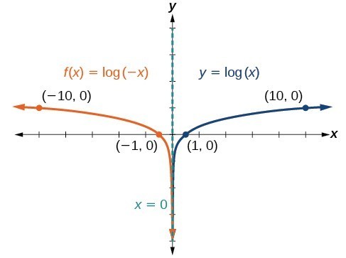 The domain is [latex]\left(-\infty ,0\right)[/latex], the range is [latex]\left(-\infty ,\infty \right)[/latex], and the vertical asymptote is x = 0.
Try It
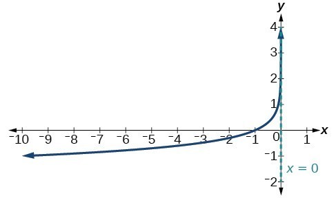
Graph [latex]f\left(x\right)=-\mathrm{log}\left(-x\right)[/latex]. State the domain, range, and asymptote.Answer:
The domain is [latex]\left(-\infty ,0\right)[/latex], the range is [latex]\left(-\infty ,\infty \right)[/latex], and the vertical asymptote is x = 0.
How To: Given a logarithmic equation, use a graphing calculator to approximate solutions
- Press [Y=]. Enter the given logarithmic equation or equations as Y1= and, if needed, Y2=.
- Press [GRAPH] to observe the graphs of the curves and use [WINDOW] to find an appropriate view of the graphs, including their point(s) of intersection.
- To find the value of x, we compute the point of intersection. Press [2ND] then [CALC]. Select "intersect" and press [ENTER] three times. The point of intersection gives the value of x for the point(s) of intersection.
Example: Approximating the Solution of a Logarithmic Equation
Solve [latex]4\mathrm{ln}\left(x\right)+1=-2\mathrm{ln}\left(x - 1\right)[/latex] graphically. Round to the nearest thousandth.Answer: Press [Y=] and enter [latex]4\mathrm{ln}\left(x\right)+1[/latex] next to Y1=. Then enter [latex]-2\mathrm{ln}\left(x - 1\right)[/latex] next to Y2=. For a window, use the values 0 to 5 for x and –10 to 10 for y. Press [GRAPH]. The graphs should intersect somewhere a little to the right of x = 1. For a better approximation, press [2ND] then [CALC]. Select [5: intersect] and press [ENTER] three times. The x-coordinate of the point of intersection is displayed as 1.3385297. (Your answer may be different if you use a different window or use a different value for Guess?) So, to the nearest thousandth, [latex]x\approx 1.339[/latex].
Try It
Solve [latex]5\mathrm{log}\left(x+2\right)=4-\mathrm{log}\left(x\right)[/latex] graphically. Round to the nearest thousandth.Answer: [latex]x\approx 3.049[/latex]
Summarizing Transformations of Logarithmic Functions
Now that we have worked with each type of transformation for the logarithmic function, we can summarize each in the table below to arrive at the general equation for transforming exponential functions.| Transformations of the Parent Function [latex]y={\mathrm{log}}_{b}\left(x\right)[/latex] | |
|---|---|
| Translation | Form |
Shift
|
[latex]y={\mathrm{log}}_{b}\left(x+c\right)+d[/latex] |
Stretch and Compression
|
[latex]y=a{\mathrm{log}}_{b}\left(x\right)[/latex] |
| Reflection about the x-axis | [latex]y=-{\mathrm{log}}_{b}\left(x\right)[/latex] |
| Reflection about the y-axis | [latex]y={\mathrm{log}}_{b}\left(-x\right)[/latex] |
| General equation for all transformations | [latex]y=a{\mathrm{log}}_{b}\left(x+c\right)+d[/latex] |
A General Note: Transformations of Logarithmic Functions
All transformations of the parent logarithmic function [latex]y={\mathrm{log}}_{b}\left(x\right)[/latex] have the form [latex-display] f\left(x\right)=a{\mathrm{log}}_{b}\left(x+c\right)+d[/latex-display] where the parent function, [latex]y={\mathrm{log}}_{b}\left(x\right),b>1[/latex], is- shifted vertically up d units.
- shifted horizontally to the left c units.
- stretched vertically by a factor of |a| if |a| > 0.
- compressed vertically by a factor of |a| if 0 < |a| < 1.
- reflected about the x-axis when a < 0.
Example: Finding the Vertical Asymptote of A LogarithmIC Function
What is the vertical asymptote of [latex]f\left(x\right)=-2{\mathrm{log}}_{3}\left(x+4\right)+5[/latex]?Answer: The vertical asymptote is at x = –4.
Analysis of the Solution
The coefficient, the base, and the upward translation do not affect the asymptote. The shift of the curve 4 units to the left shifts the vertical asymptote to x = –4.Try It
What is the vertical asymptote of [latex]f\left(x\right)=3+\mathrm{ln}\left(x - 1\right)[/latex]?Answer: [latex]x=1[/latex]
tip for success
In the example below, you'll write a common logarithmic function for the graph shown. Remember that all the functions studied in this course possess the characteristic that every point contained on the graph of a function satisfies the equation of the function. As you have done before, begin with the form of a transformed logarithm function, [latex]f(x)=a\text{log}(x+c)+d[/latex], then fill in the parts you can discern from the graph.- Find the horizontal shift by locating the vertical asymptote.
- Examine the shape of the graph to see if it has been reflected.
- Once you have filled in what you know, substitute one or more points in integer coordinates if possible to solve for any remaining unknowns.
- Remember that if there are more than one unknown, you'll need more than one point and more than one equation to solve for all the unknowns.
Example: Finding the Equation from a Graph
Find a possible equation for the common logarithmic function graphed below.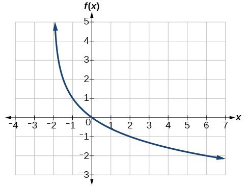
Answer: This graph has a vertical asymptote at x = –2 and has been vertically reflected. We do not know yet the vertical shift or the vertical stretch. We know so far that the equation will have the form:
[latex]f\left(x\right)=-a\mathrm{log}\left(x+2\right)+k[/latex]
It appears the graph passes through the points [latex]\left(-1,1\right)[/latex] and [latex]\left(2,-1\right)[/latex]. Substituting [latex]\left(-1,1\right)[/latex],[latex]\begin{array}{llll}1=-a\mathrm{log}\left(-1+2\right)+k\hfill & \text{Substitute }\left(-1,1\right).\hfill \\ 1=-a\mathrm{log}\left(1\right)+k\hfill & \text{Arithmetic}.\hfill \\ 1=k\hfill & \text{log(1)}=0.\hfill \end{array}[/latex]
Next, substituting [latex]\left(2,-1\right)[/latex],[latex]\begin{array}{llllll}-1=-a\mathrm{log}\left(2+2\right)+1\hfill & \hfill & \text{Plug in }\left(2,-1\right).\hfill \\ -2=-a\mathrm{log}\left(4\right)\hfill & \hfill & \text{Arithmetic}.\hfill \\ \text{ }a=\frac{2}{\mathrm{log}\left(4\right)}\hfill & \hfill & \text{Solve for }a.\hfill \end{array}[/latex]
This gives us the equation [latex]f\left(x\right)=-\frac{2}{\mathrm{log}\left(4\right)}\mathrm{log}\left(x+2\right)+1[/latex].Analysis of the Solution
We can verify this answer by comparing the function values in the table below with the points on the graph in this example.| x | −1 | 0 | 1 | 2 | 3 |
| f(x) | 1 | 0 | −0.58496 | −1 | −1.3219 |
| x | 4 | 5 | 6 | 7 | 8 |
| f(x) | −1.5850 | −1.8074 | −2 | −2.1699 | −2.3219 |
Try It
Give the equation of the natural logarithm graphed below.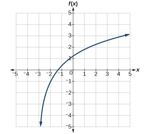
Answer: [latex]f\left(x\right)=2\mathrm{ln}\left(x+3\right)-1[/latex]
Q & A
Is it possible to tell the domain and range and describe the end behavior of a function just by looking at the graph? Yes if we know the function is a general logarithmic function. For example, look at the graph in the previous example. The graph approaches x = –3 (or thereabouts) more and more closely, so x = –3 is, or is very close to, the vertical asymptote. It approaches from the right, so the domain is all points to the right, [latex]\left\{x|x>-3\right\}[/latex]. The range, as with all general logarithmic functions, is all real numbers. And we can see the end behavior because the graph goes down as it goes left and up as it goes right. The end behavior is as [latex]x\to -{3}^{+},f\left(x\right)\to -\infty [/latex] and as [latex]x\to \infty ,f\left(x\right)\to \infty [/latex].Licenses & Attributions
CC licensed content, Original
- Revision and Adaptation. Provided by: Lumen Learning License: CC BY: Attribution.
- Reflections of Logarithmic Functions Interactive. Authored by: Lumen Learning. Located at: https://www.desmos.com/calculator/5qmaorrlst. License: Public Domain: No Known Copyright.
- Vertical Stretch and Compression of a Logarithmic Function Interactive. Authored by: Lumen Learning. Located at: https://www.desmos.com/calculator/arlodqq7be. License: Public Domain: No Known Copyright.
CC licensed content, Shared previously
- College Algebra. Provided by: OpenStax Authored by: Abramson, Jay et al.. Located at: https://openstax.org/books/college-algebra/pages/1-introduction-to-prerequisites. License: CC BY: Attribution. License terms: Download for free at http://cnx.org/contents/[email protected].
