
Multiplicity and Turning Points
Learning Objectives
- Identify zeros of polynomial functions with even and odd multiplicity
- Use the degree of a polynomial to determine the number of turning points of its graph
 Identifying the behavior of the graph at an x-intercept by examining the multiplicity of the zero.
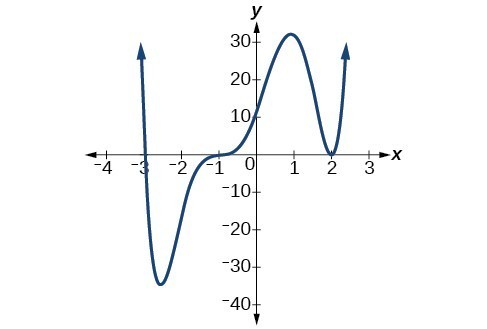
[latex]{\left(x - 2\right)}^{2}=\left(x - 2\right)\left(x - 2\right)[/latex]
The factor is repeated, that is, the factor [latex]\left(x - 2\right)[/latex] appears twice. The number of times a given factor appears in the factored form of the equation of a polynomial is called the multiplicity. The zero associated with this factor, [latex]x=2[/latex], has multiplicity 2 because the factor [latex]\left(x - 2\right)[/latex] occurs twice. The x-intercept [latex]x=-1[/latex] is the repeated solution of factor [latex]{\left(x+1\right)}^{3}=0[/latex]. The graph passes through the axis at the intercept, but flattens out a bit first. This factor is cubic (degree 3), so the behavior near the intercept is like that of a cubic—with the same S-shape near the intercept as the toolkit function [latex]f\left(x\right)={x}^{3}[/latex]. We call this a triple zero, or a zero with multiplicity 3. For zeros with even multiplicities, the graphs touch or are tangent to the x-axis. For zeros with odd multiplicities, the graphs cross or intersect the x-axis. See the figure below for examples of graphs of polynomial functions with multiplicity 1, 2, and 3.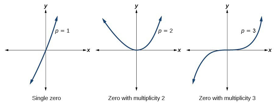 For higher even powers, such as 4, 6, and 8, the graph will still touch and bounce off of the horizontal axis but, for each increasing even power, the graph will appear flatter as it approaches and leaves the x-axis.
For higher odd powers, such as 5, 7, and 9, the graph will still cross through the horizontal axis, but for each increasing odd power, the graph will appear flatter as it approaches and leaves the x-axis.
For higher even powers, such as 4, 6, and 8, the graph will still touch and bounce off of the horizontal axis but, for each increasing even power, the graph will appear flatter as it approaches and leaves the x-axis.
For higher odd powers, such as 5, 7, and 9, the graph will still cross through the horizontal axis, but for each increasing odd power, the graph will appear flatter as it approaches and leaves the x-axis.
A General Note: Graphical Behavior of Polynomials at x-Intercepts
If a polynomial contains a factor of the form [latex]{\left(x-h\right)}^{p}[/latex], the behavior near the x-intercept h is determined by the power p. We say that [latex]x=h[/latex] is a zero of multiplicity p. The graph of a polynomial function will touch the x-axis at zeros with even multiplicities. The graph will cross the x-axis at zeros with odd multiplicities. The sum of the multiplicities is the degree of the polynomial function.How To: Given a graph of a polynomial function of degree n, identify the zeros and their multiplicities.
- If the graph crosses the x-axis and appears almost linear at the intercept, it is a single zero.
- If the graph touches the x-axis and bounces off of the axis, it is a zero with even multiplicity.
- If the graph crosses the x-axis at a zero, it is a zero with odd multiplicity.
- The sum of the multiplicities is n.
Example: Identifying Zeros and Their Multiplicities
Use the graph of the function of degree 6 to identify the zeros of the function and their possible multiplicities.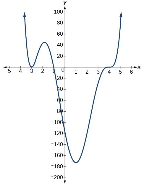
Answer: The polynomial function is of degree n. The sum of the multiplicities must be n. Starting from the left, the first zero occurs at [latex]x=-3[/latex]. The graph touches the x-axis, so the multiplicity of the zero must be even. The zero of –3 has multiplicity 2. The next zero occurs at [latex]x=-1[/latex]. The graph looks almost linear at this point. This is a single zero of multiplicity 1. The last zero occurs at [latex]x=4[/latex]. The graph crosses the x-axis, so the multiplicity of the zero must be odd. We know that the multiplicity is likely 3 and that the sum of the multiplicities is likely 6.
Try It
Use the graph of the function of degree 5 to identify the zeros of the function and their multiplicities.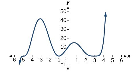
Answer: The graph has a zero of –5 with multiplicity 1, a zero of –1 with multiplicity 2, and a zero of 3 with even multiplicity.
Try It
Use the graph below to find the zeros of the degree 6 function, and their multiplicities. https://www.desmos.com/calculator/rvbhedb5tb [practice-area rows="2"][/practice-area]Answer:
| Zero | Multiplicity |
| [latex](-3,0)[/latex] | 1 |
| [latex](-2,0)[/latex] | 2 |
| [latex](1,0)[/latex] | 3 |
Determine end behavior
As we have already learned, the behavior of a graph of a polynomial function of the form[latex]f\left(x\right)={a}_{n}{x}^{n}+{a}_{n - 1}{x}^{n - 1}+...+{a}_{1}x+{a}_{0}[/latex]
will either ultimately rise or fall as x increases without bound and will either rise or fall as x decreases without bound. This is because for very large inputs, say 100 or 1,000, the leading term dominates the size of the output. The same is true for very small inputs, say –100 or –1,000. Recall that we call this behavior the end behavior of a function. As we pointed out when discussing quadratic equations, when the leading term of a polynomial function, [latex]{a}_{n}{x}^{n}[/latex], is an even power function, as x increases or decreases without bound, [latex]f\left(x\right)[/latex] increases without bound. When the leading term is an odd power function, as x decreases without bound, [latex]f\left(x\right)[/latex] also decreases without bound; as x increases without bound, [latex]f\left(x\right)[/latex] also increases without bound. If the leading term is negative, it will change the direction of the end behavior. The table below summarizes all four cases.| Even Degree | Odd Degree |
|---|---|
 |
 |
 |
 |
Licenses & Attributions
CC licensed content, Original
- Question ID 121830. Authored by: Lumen Learning. License: Other. License terms: IMathAS Community License CC-BY + GPL.
- Revision and Adaptation. Provided by: Lumen Learning License: CC BY: Attribution.
CC licensed content, Shared previously
- Question ID 29470. Authored by: Caren McClure. License: Other. License terms: IMathAS Community License CC-BY + GPL.
- College Algebra. Provided by: OpenStax Authored by: Abramson, Jay et al.. Located at: https://openstax.org/books/college-algebra/pages/1-introduction-to-prerequisites. License: CC BY: Attribution. License terms: Download for free at http://cnx.org/contents/[email protected].
