
Rates of Change and Behavior of Graphs
Gasoline costs have experienced some wild fluctuations over the last several decades. The table below[footnote]http://www.eia.gov/totalenergy/data/annual/showtext.cfm?t=ptb0524. Accessed 3/5/2014.[/footnote] lists the average cost, in dollars, of a gallon of gasoline for the years 2005–2012. The cost of gasoline can be considered as a function of year.| [latex]y[/latex] | 2005 | 2006 | 2007 | 2008 | 2009 | 2010 | 2011 | 2012 |
| [latex]C\left(y\right)[/latex] | 2.31 | 2.62 | 2.84 | 3.30 | 2.41 | 2.84 | 3.58 | 3.68 |
Rates of Change
Gasoline costs have experienced some wild fluctuations over the last several decades. The table below[footnote]http://www.eia.gov/totalenergy/data/annual/showtext.cfm?t=ptb0524. Accessed 3/5/2014.[/footnote] lists the average cost, in dollars, of a gallon of gasoline for the years 2005–2012. The cost of gasoline can be considered as a function of year.| [latex]y[/latex] | 2005 | 2006 | 2007 | 2008 | 2009 | 2010 | 2011 | 2012 |
| [latex]C\left(y\right)[/latex] | 2.31 | 2.62 | 2.84 | 3.30 | 2.41 | 2.84 | 3.58 | 3.68 |
| [latex]y[/latex] | 2005 | 2006 | 2007 | 2008 | 2009 | 2010 | 2011 | 2012 |
| [latex]C\left(y\right)[/latex] | 2.31 | 2.62 | 2.84 | 3.30 | 2.41 | 2.84 | 3.58 | 3.68 |
[latex]\begin{array}{l}\text{Average rate of change}=\frac{\text{Change in output}}{\text{Change in input}}\\\,\,\,\,\,\,\,\,\,\,\,\,\,\,\,\,\,\,\,\,\,\,\,\,\,\,\,\,\,\,\,\,\,\,\,\,\,\,\,\,\,\,\,\,\,\,\,\,\,\,\,\,\,\,\,\,\,\,\,\,\,=\frac{\Delta y}{\Delta x}\\\,\,\,\,\,\,\,\,\,\,\,\,\,\,\,\,\,\,\,\,\,\,\,\,\,\,\,\,\,\,\,\,\,\,\,\,\,\,\,\,\,\,\,\,\,\,\,\,\,\,\,\,\,\,\,\,\,\,\,\,\,=\frac{{y}_{2}-{y}_{1}}{{x}_{2}-{x}_{1}}\\\,\,\,\,\,\,\,\,\,\,\,\,\,\,\,\,\,\,\,\,\,\,\,\,\,\,\,\,\,\,\,\,\,\,\,\,\,\,\,\,\,\,\,\,\,\,\,\,\,\,\,\,\,\,\,\,\,\,\,\,\,=\frac{f\left({x}_{2}\right)-f\left({x}_{1}\right)}{{x}_{2}-{x}_{1}}\end{array}[/latex]
The Greek letter [latex]\Delta [/latex] (delta) signifies the change in a quantity; we read the ratio as "delta-y over delta-x" or "the change in [latex]y[/latex] divided by the change in [latex]x[/latex]." Occasionally we write [latex]\Delta f[/latex] instead of [latex]\Delta y[/latex], which still represents the change in the function’s output value resulting from a change to its input value. It does not mean we are changing the function into some other function. In our example, the gasoline price increased by $1.37 from 2005 to 2012. Over 7 years, the average rate of change was[latex]\frac{\Delta y}{\Delta x}=\frac{{1.37}}{\text{7 years}}\approx 0.196\text{ dollars per year}[/latex]
On average, the price of gas increased by about 19.6¢ each year. Other examples of rates of change include:- A population of rats increasing by 40 rats per week
- A car traveling 68 miles per hour (distance traveled changes by 68 miles each hour as time passes)
- A car driving 27 miles per gallon (distance traveled changes by 27 miles for each gallon)
- The current through an electrical circuit increasing by 0.125 amperes for every volt of increased voltage
- The amount of money in a college account decreasing by $4,000 per quarter
A General Note: Rate of Change
A rate of change describes how an output quantity changes relative to the change in the input quantity. The units on a rate of change are "output units per input units." The average rate of change between two input values is the total change of the function values (output values) divided by the change in the input values.[latex]\frac{\Delta y}{\Delta x}=\frac{f\left({x}_{2}\right)-f\left({x}_{1}\right)}{{x}_{2}-{x}_{1}}[/latex]
How To: Given the value of a function at different points, calculate the average rate of change of a function for the interval between two values [latex]{x}_{1}[/latex] and [latex]{x}_{2}[/latex].
- Calculate the difference [latex]{y}_{2}-{y}_{1}=\Delta y[/latex].
- Calculate the difference [latex]{x}_{2}-{x}_{1}=\Delta x[/latex].
- Find the ratio [latex]\frac{\Delta y}{\Delta x}[/latex].
Example: Computing an Average Rate of Change
Using the data in the table below, find the average rate of change of the price of gasoline between 2007 and 2009.| [latex]y[/latex] | 2005 | 2006 | 2007 | 2008 | 2009 | 2010 | 2011 | 2012 |
| [latex]C\left(y\right)[/latex] | 2.31 | 2.62 | 2.84 | 3.30 | 2.41 | 2.84 | 3.58 | 3.68 |
Answer: In 2007, the price of gasoline was $2.84. In 2009, the cost was $2.41. The average rate of change is
[latex]\begin{array}{l}\frac{\Delta y}{\Delta x}=\frac{{y}_{2}-{y}_{1}}{{x}_{2}-{x}_{1}}\\\,\,\,\,\,\,\,\,\,\,=\frac{2.41-2.84}{2009 - 2007}\\\,\,\,\,\,\,\,\,\,\,=\frac{-0.43}{2\text{ years}}\\\,\,\,\,\,\,\,\,\,\,={-0.22}\text{ per year}\end{array}[/latex]
Analysis of the Solution
Note that a decrease is expressed by a negative change or "negative increase." A rate of change is negative when the output decreases as the input increases or when the output increases as the input decreases. The following video provides another example of how to find the average rate of change between two points from a table of values.Try It
Using the data in the table below, find the average rate of change between 2005 and 2010.| [latex]y[/latex] | 2005 | 2006 | 2007 | 2008 | 2009 | 2010 | 2011 | 2012 |
| [latex]C\left(y\right)[/latex] | 2.31 | 2.62 | 2.84 | 3.30 | 2.41 | 2.84 | 3.58 | 3.68 |
Answer: [latex]\frac{$2.84-$2.31}{5\text{ years}}=\frac{$0.53}{5\text{ years}}=$0.106[/latex] per year.
Example: Computing Average Rate of Change from a Graph
Given the function [latex]g\left(t\right)[/latex], find the average rate of change on the interval [latex]\left[-1,2\right][/latex].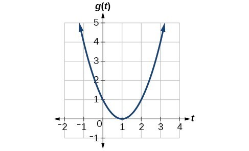
Answer:
 At [latex]t=-1[/latex], the graph shows [latex]g\left(-1\right)=4[/latex]. At [latex]t=2[/latex], the graph shows [latex]g\left(2\right)=1[/latex].
The horizontal change [latex]\Delta t=3[/latex] is shown by the red arrow, and the vertical change [latex]\Delta g\left(t\right)=-3[/latex] is shown by the turquoise arrow. The output changes by –3 while the input changes by 3, giving an average rate of change of
At [latex]t=-1[/latex], the graph shows [latex]g\left(-1\right)=4[/latex]. At [latex]t=2[/latex], the graph shows [latex]g\left(2\right)=1[/latex].
The horizontal change [latex]\Delta t=3[/latex] is shown by the red arrow, and the vertical change [latex]\Delta g\left(t\right)=-3[/latex] is shown by the turquoise arrow. The output changes by –3 while the input changes by 3, giving an average rate of change of
[latex]\frac{1 - 4}{2-\left(-1\right)}=\frac{-3}{3}=-1[/latex]
Analysis of the Solution
Note that the order we choose is very important. If, for example, we use [latex]\frac{{y}_{2}-{y}_{1}}{{x}_{1}-{x}_{2}}[/latex], we will not get the correct answer. Decide which point will be 1 and which point will be 2, and keep the coordinates fixed as [latex]\left({x}_{1},{y}_{1}\right)[/latex] and [latex]\left({x}_{2},{y}_{2}\right)[/latex].Example: Finding the Average Rate of Change of a Force
The electrostatic force [latex]F[/latex], measured in newtons, between two charged particles can be related to the distance between the particles [latex]d[/latex], in centimeters, by the formula [latex]F\left(d\right)=\frac{2}{{d}^{2}}[/latex]. Find the average rate of change of force if the distance between the particles is increased from 2 cm to 6 cm.Answer: We are computing the average rate of change of [latex]F\left(d\right)=\frac{2}{{d}^{2}}[/latex] on the interval [latex]\left[2,6\right][/latex].
[latex]\begin{array}{l}\text{Average rate of change.}=\frac{F\left(6\right)-F\left(2\right)}{6 - 2}\\ \,\,\,\,\,\,\,\,\,\,\,\,\,\,\,\,\,\,\,\,\,\,\,\,\,\,\,\,\,\,\,\,\,\,\,\,\,\,\,\,\,\,\,\,\,\,\,\,\,\,\,\,\,\,\,\,\,\,\,\,\,\,\,=\frac{\frac{2}{{6}^{2}}-\frac{2}{{2}^{2}}}{6 - 2} \,\,\,\,\,\,\,\,\,\,\,\,\,\text{Simplify.} \\\,\,\,\,\,\,\,\,\,\,\,\,\,\,\,\,\,\,\,\,\,\,\,\,\,\,\,\,\,\,\,\,\,\,\,\,\,\,\,\,\,\,\,\,\,\,\,\,\,\,\,\,\,\,\,\,\,\,\,\,\,\,\,=\frac{\frac{2}{36}-\frac{2}{4}}{4}\\\,\,\,\,\,\,\,\,\,\,\,\,\,\,\,\,\,\,\,\,\,\,\,\,\,\,\,\,\,\,\,\,\,\,\,\,\,\,\,\,\,\,\,\,\,\,\,\,\,\,\,\,\,\,\,\,\,\,\,\,\,\,\,=\frac{-\frac{16}{36}}{4}\,\,\,\,\,\,\,\,\,\,\,\,\,\,\,\,\,\,\,\text{Combine numerator terms.}\\\,\,\,\,\,\,\,\,\,\,\,\,\,\,\,\,\,\,\,\,\,\,\,\,\,\,\,\,\,\,\,\,\,\,\,\,\,\,\,\,\,\,\,\,\,\,\,\,\,\,\,\,\,\,\,\,\,\,\,\,\,\,\,=-\frac{1}{9}\,\,\,\,\,\,\,\,\,\,\,\,\,\,\,\,\,\,\,\,\text{Simplify.}\end{array}[/latex]
The average rate of change is [latex]-\frac{1}{9}[/latex] newton per centimeter.Example: Finding an Average Rate of Change as an Expression
Find the average rate of change of [latex]g\left(t\right)={t}^{2}+3t+1[/latex] on the interval [latex]\left[0,a\right][/latex]. The answer will be an expression involving [latex]a[/latex].Answer: We use the average rate of change formula.
[latex]\begin{array}{l}\text{Average rate of change}=\frac{g\left(a\right)-g\left(0\right)}{a - 0}\text{Evaluate.}\\\,\,\,\,\,\,\,\,\,\,\,\,\,\,\,\,\,\,\,\,\,\,\,\,\,\,\,\,\,\,\,\,\,\,\,\,\,\,\,\,\,\,\,\,\,\,\,\,\,\,\,\,\,\,\,\,\,\,\,\,\,=\frac{\left({a}^{2}+3a+1\right)-\left({0}^{2}+3\left(0\right)+1\right)}{a - 0}\,\,\,\,\,\,\,\,\,\,\,\,\,\,\,\,\text{Simplify.}\\\,\,\,\,\,\,\,\,\,\,\,\,\,\,\,\,\,\,\,\,\,\,\,\,\,\,\,\,\,\,\,\,\,\,\,\,\,\,\,\,\,\,\,\,\,\,\,\,\,\,\,\,\,\,\,\,\,\,\,\,\,=\frac{{a}^{2}+3a+1 - 1}{a}\,\,\,\,\,\,\,\,\,\,\,\,\,\,\,\,\,\,\,\,\,\,\,\,\,\,\,\,\,\,\,\,\,\,\,\,\,\,\,\,\,\,\text{Simplify and factor.}\\\,\,\,\,\,\,\,\,\,\,\,\,\,\,\,\,\,\,\,\,\,\,\,\,\,\,\,\,\,\,\,\,\,\,\,\,\,\,\,\,\,\,\,\,\,\,\,\,\,\,\,\,\,\,\,\,\,\,\,\,\,=\frac{a\left(a+3\right)}{a}\,\,\,\,\,\,\,\,\,\,\,\,\,\,\,\,\,\,\,\,\,\,\,\,\,\,\,\,\,\,\,\,\,\,\,\,\,\,\,\,\,\,\,\,\,\,\,\,\,\,\,\text{Divide by the common factor }a.\\\,\,\,\,\,\,\,\,\,\,\,\,\,\,\,\,\,\,\,\,\,\,\,\,\,\,\,\,\,\,\,\,\,\,\,\,\,\,\,\,\,\,\,\,\,\,\,\,\,\,\,\,\,\,\,\,\,\,\,\,\,=a+3\end{array}[/latex]
This result tells us the average rate of change in terms of [latex]a[/latex] between [latex]t=0[/latex] and any other point [latex]t=a[/latex]. For example, on the interval [latex]\left[0,5\right][/latex], the average rate of change would be [latex]5+3=8[/latex].Try It
Find the average rate of change of [latex]f\left(x\right)={x}^{2}+2x - 8[/latex] on the interval [latex]\left[5,a\right][/latex].Answer: [latex]a+7[/latex]
Behaviors of Functions
As part of exploring how functions change, we can identify intervals over which the function is changing in specific ways. We say that a function is increasing on an interval if the function values increase as the input values increase within that interval. Similarly, a function is decreasing on an interval if the function values decrease as the input values increase over that interval. The average rate of change of an increasing function is positive, and the average rate of change of a decreasing function is negative. The graph below shows examples of increasing and decreasing intervals on a function.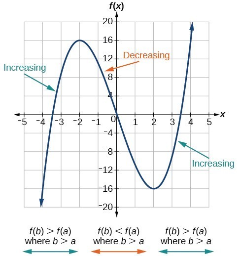 The function [latex]f\left(x\right)={x}^{3}-12x[/latex] is increasing on [latex]\left(-\infty \text{,}-\text{2}\right){{\cup }^{\text{ }}}^{\text{ }}\left(2,\infty \right)[/latex] and is decreasing on [latex]\left(-2\text{,}2\right)[/latex].
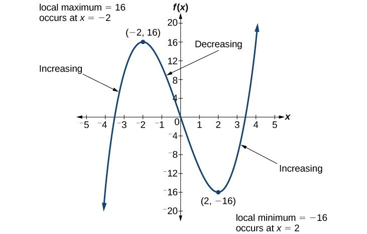 To locate the local maxima and minima from a graph, we need to observe the graph to determine where the graph attains its highest and lowest points, respectively, within an open interval. Like the summit of a roller coaster, the graph of a function is higher at a local maximum than at nearby points on both sides. The graph will also be lower at a local minimum than at neighboring points. The graph below illustrates these ideas for a local maximum.
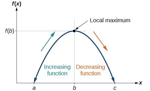 Definition of a local maximum.
A General Note: Local Minima and Local Maxima
A function [latex]f[/latex] is an increasing function on an open interval if [latex]f\left(b\right)>f\left(a\right)[/latex] for any two input values [latex]a[/latex] and [latex]b[/latex] in the given interval where [latex]b>a[/latex]. A function [latex]f[/latex] is a decreasing function on an open interval if [latex]f\left(b\right)<f\left(a\right)[/latex] for any two input values [latex]a[/latex] and [latex]b[/latex] in the given interval where [latex]b>a[/latex]. A function [latex]f[/latex] has a local maximum at [latex]x=b[/latex] if there exists an interval [latex]\left(a,c\right)[/latex] with [latex]a<b<c[/latex] such that, for any [latex]x[/latex] in the interval [latex]\left(a,c\right)[/latex], [latex]f\left(x\right)\le f\left(b\right)[/latex]. Likewise, [latex]f[/latex] has a local minimum at [latex]x=b[/latex] if there exists an interval [latex]\left(a,c\right)[/latex] with [latex]a<b<c[/latex] such that, for any [latex]x[/latex] in the interval [latex]\left(a,c\right)[/latex], [latex]f\left(x\right)\ge f\left(b\right)[/latex].Example: Finding Increasing and Decreasing Intervals on a Graph
Given the function [latex]p\left(t\right)[/latex] in the graph below, identify the intervals on which the function appears to be increasing.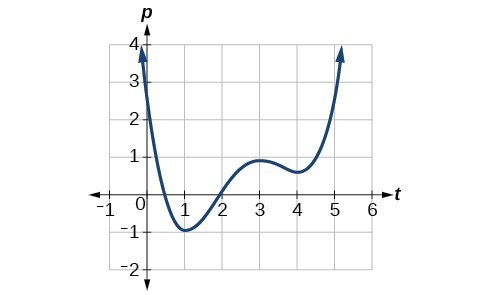
Answer: We see that the function is not constant on any interval. The function is increasing where it slants upward as we move to the right and decreasing where it slants downward as we move to the right. The function appears to be increasing from [latex]t=1[/latex] to [latex]t=3[/latex] and from [latex]t=4[/latex] on. In interval notation, we would say the function appears to be increasing on the interval (1,3) and the interval [latex]\left(4,\infty \right)[/latex].
Analysis of the Solution
Notice in this example that we used open intervals (intervals that do not include the endpoints), because the function is neither increasing nor decreasing at [latex]t=1[/latex] , [latex]t=3[/latex] , and [latex]t=4[/latex] . These points are the local extrema (two minima and a maximum).Example: Finding Local Maxima and Minima from a Graph
For the function [latex]f[/latex] whose graph is shown below, find all local maxima and minima.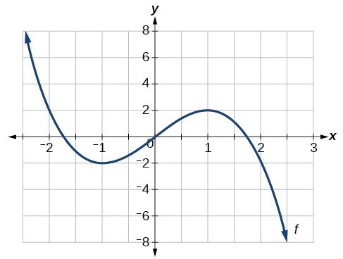
Answer: Observe the graph of [latex]f[/latex]. The graph attains a local maximum at [latex]x=1[/latex] because it is the highest point in an open interval around [latex]x=1[/latex]. The local maximum is the [latex]y[/latex] -coordinate at [latex]x=1[/latex], which is [latex]2[/latex]. The graph attains a local minimum at [latex]\text{ }x=-1\text{ }[/latex] because it is the lowest point in an open interval around [latex]x=-1[/latex]. The local minimum is the y-coordinate at [latex]x=-1[/latex], which is [latex]-2[/latex].
Analyzing the Toolkit Functions for Increasing or Decreasing Intervals
We will now return to our toolkit functions and discuss their graphical behavior in the table below.| Function | Increasing/Decreasing | Example |
|---|---|---|
| Constant Function [latex]f\left(x\right)={c}[/latex] | Neither increasing nor decreasing | 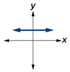 |
| Identity Function [latex]f\left(x\right)={x}[/latex] | Increasing | 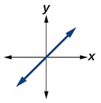 |
| Quadratic Function [latex]f\left(x\right)={x}^{2}[/latex] | Increasing on [latex]\left(0,\infty\right)[/latex] Decreasing on [latex]\left(-\infty,0\right)[/latex] Minimum at [latex]x=0[/latex] | 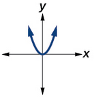 |
| Cubic Function [latex]f\left(x\right)={x}^{3}[/latex] | Increasing | 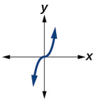 |
| Reciprocal [latex]f\left(x\right)=\frac{1}{x}[/latex] | Decreasing [latex]\left(-\infty,0\right)\cup\left(0,\infty\right)[/latex] | 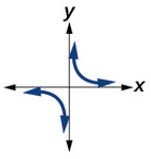 |
| Reciprocal Squared [latex]f\left(x\right)=\frac{1}{{x}^{2}}[/latex] | Increasing on [latex]\left(-\infty,0\right)[/latex] Decreasing on [latex]\left(0,\infty\right)[/latex] | 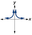 |
| Cube Root [latex]f\left(x\right)=\sqrt[3]{x}[/latex] | Increasing | 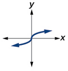 |
| Square Root [latex]f\left(x\right)=\sqrt{x}[/latex] | Increasing on [latex]\left(0,\infty\right)[/latex] | 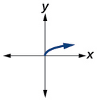 |
| Absolute Value [latex]f\left(x\right)=|x|[/latex] | Increasing on [latex]\left(0,\infty\right)[/latex] Decreasing on [latex]\left(-\infty,0\right)[/latex] | 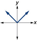 |
Use a graph to locate the absolute maximum and absolute minimum of a function
There is a difference between locating the highest and lowest points on a graph in a region around an open interval (locally) and locating the highest and lowest points on the graph for the entire domain. The [latex]y\text{-}[/latex] coordinates (output) at the highest and lowest points are called the absolute maximum and absolute minimum, respectively. To locate absolute maxima and minima from a graph, we need to observe the graph to determine where the graph attains it highest and lowest points on the domain of the function.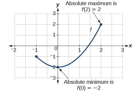 Not every function has an absolute maximum or minimum value. The toolkit function [latex]f\left(x\right)={x}^{3}[/latex] is one such function.
A General Note: Absolute Maxima and Minima
The absolute maximum of [latex]f[/latex] at [latex]x=c[/latex] is [latex]f\left(c\right)[/latex] where [latex]f\left(c\right)\ge f\left(x\right)[/latex] for all [latex]x[/latex] in the domain of [latex]f[/latex]. The absolute minimum of [latex]f[/latex] at [latex]x=d[/latex] is [latex]f\left(d\right)[/latex] where [latex]f\left(d\right)\le f\left(x\right)[/latex] for all [latex]x[/latex] in the domain of [latex]f[/latex].Example: Finding Absolute Maxima and Minima from a Graph
For the function [latex]f[/latex] shown below, find all absolute maxima and minima.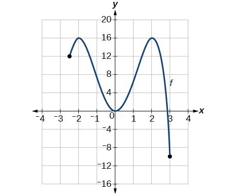
Answer: Observe the graph of [latex]f[/latex]. The graph attains an absolute maximum in two locations, [latex]x=-2[/latex] and [latex]x=2[/latex], because at these locations, the graph attains its highest point on the domain of the function. The absolute maximum is the y-coordinate at [latex]x=-2[/latex] and [latex]x=2[/latex], which is [latex]16[/latex]. The graph attains an absolute minimum at [latex]x=3[/latex], because it is the lowest point on the domain of the function’s graph. The absolute minimum is the y-coordinate at [latex]x=3[/latex], which is [latex]-10[/latex].
Key Equations
| Average rate of change | [latex]\frac{\Delta y}{\Delta x}=\frac{f\left({x}_{2}\right)-f\left({x}_{1}\right)}{{x}_{2}-{x}_{1}}[/latex] |
Key Concepts
- A rate of change relates a change in an output quantity to a change in an input quantity. The average rate of change is determined using only the beginning and ending data.
- Identifying points that mark the interval on a graph can be used to find the average rate of change.
- Comparing pairs of input and output values in a table can also be used to find the average rate of change.
- An average rate of change can also be computed by determining the function values at the endpoints of an interval described by a formula.
- The average rate of change can sometimes be determined as an expression.
- A function is increasing where its rate of change is positive and decreasing where its rate of change is negative.
- A local maximum is where a function changes from increasing to decreasing and has an output value larger (more positive or less negative) than output values at neighboring input values.
- A local minimum is where the function changes from decreasing to increasing (as the input increases) and has an output value smaller (more negative or less positive) than output values at neighboring input values.
- Minima and maxima are also called extrema.
- We can find local extrema from a graph.
- The highest and lowest points on a graph indicate the maxima and minima.
Glossary
- absolute maximum
- the greatest value of a function over an interval
- absolute minimum
- the lowest value of a function over an interval
- average rate of change
- the difference in the output values of a function found for two values of the input divided by the difference between the inputs
- decreasing function
- a function is decreasing in some open interval if [latex]f\left(b\right)<f\left(a\right)[/latex] for any two input values [latex]a[/latex] and [latex]b[/latex] in the given interval where [latex]b>a[/latex]
- increasing function
- a function is increasing in some open interval if [latex]f\left(b\right)>f\left(a\right)[/latex] for any two input values [latex]a[/latex] and [latex]b[/latex] in the given interval where [latex]b>a[/latex]
- local extrema
- collectively, all of a function's local maxima and minima
- local maximum
- a value of the input where a function changes from increasing to decreasing as the input value increases.
- local minimum
- a value of the input where a function changes from decreasing to increasing as the input value increases.
- rate of change
- the change of an output quantity relative to the change of the input quantity
Licenses & Attributions
CC licensed content, Original
- Revision and Adaptation. Provided by: Lumen Learning License: CC BY: Attribution.
- Question ID 111818. Authored by: Lumen Learning. License: CC BY: Attribution. License terms: IMathAS Community License CC-BY + GPL.
CC licensed content, Shared previously
- College Algebra. Provided by: OpenStax Authored by: Abramson, Jay et al.. Located at: https://openstax.org/books/college-algebra/pages/1-introduction-to-prerequisites. License: CC BY: Attribution. License terms: Download for free at http://cnx.org/contents/[email protected].
- Ex: Find the Average Rate of Change From a Table - Temperatures. Authored by: Mathispower4u. License: All Rights Reserved. License terms: Standard YouTube License.
- Question ID 1731, 1732, 1733, 4083, 4084. Authored by: Lippman, David. License: CC BY: Attribution. License terms: IMathAS Community License CC-BY + GPL.
- Question ID 74150. Authored by: Nearing,Daniel, mb Meacham, William. License: CC BY: Attribution. License terms: IMathAS Community License CC-BY + GPL.
- Question ID 16233. Authored by: Sousa, James, mb Lippman, David. License: CC BY: Attribution. License terms: IMathAS Community License CC-BY + GPL.
- Question ID 32572, 32571. Authored by: Smart, Jim. License: CC BY: Attribution. License terms: IMathAS Community License CC-BY + GPL.
